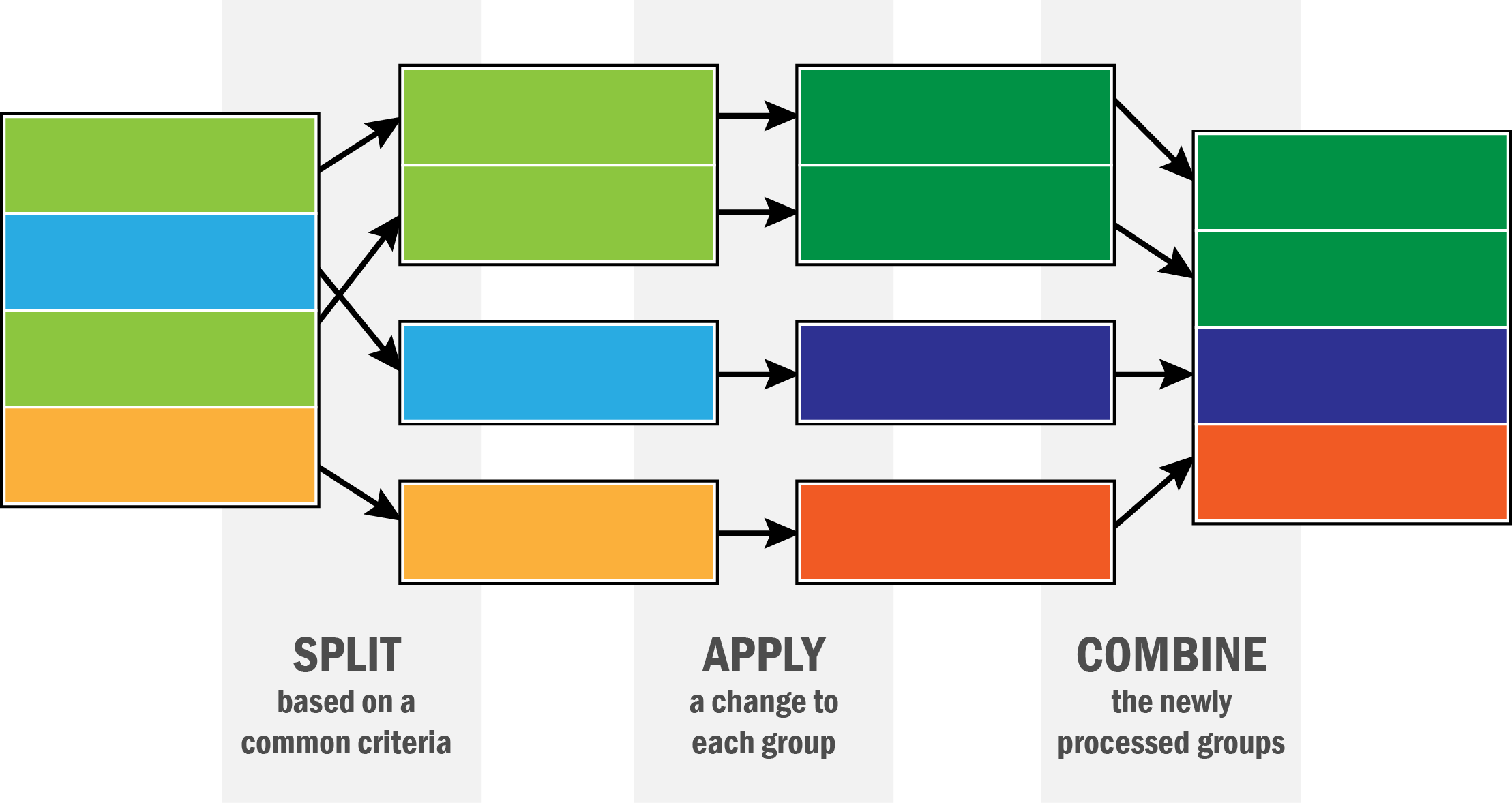
5.1 Split-apply-combine, a.k.a. MapReduce
The split-apply-combine is a powerful paradigm for understanding subgroups within a dataset. The basic idea is that you split the data into pieces based on values of some variables, do something (the same thing) to each piece, and then stitch the results back together.
For example, in the mtcars data, we might want to know what the average mpg is by the number of cylinders. The way to do this is:
mtcars1 %>%
  group_by(cyl) %>%
  summarize(mpg_mean = mean(mpg))
## # A tibble: 3 x 2
## cyl mpg_mean
## <fct> <dbl>
## 1 4 26.7
## 2 6 19.7
## 3 8 15.1Once again, the scoped versions of summarize will also work in this pipe
mtcars1 %>%
  group_by(cyl) %>%
  summarize_if(is.numeric, mean)
## # A tibble: 3 x 7
## cyl mpg disp hp drat wt qsec
## <fct> <dbl> <dbl> <dbl> <dbl> <dbl> <dbl>
## 1 4 26.7 105. 82.6 4.07 2.29 19.1
## 2 6 19.7 183. 122. 3.59 3.12 18.0
## 3 8 15.1 353. 209. 3.23 4.00 16.8Let’s go a bit further and compute the medians as well.
mtcars1 %>%
  group_by(cyl) %>%
  summarize_if(is.numeric, list('mean'= mean, 'median' = median))
## # A tibble: 3 x 13
## cyl mpg_mean disp_mean hp_mean drat_mean wt_mean qsec_mean mpg_median
## <fct> <dbl> <dbl> <dbl> <dbl> <dbl> <dbl> <dbl>
## 1 4 26.7 105. 82.6 4.07 2.29 19.1 26
## 2 6 19.7 183. 122. 3.59 3.12 18.0 19.7
## 3 8 15.1 353. 209. 3.23 4.00 16.8 15.2
## # … with 5 more variables: disp_median <dbl>, hp_median <dbl>,
## # drat_median <dbl>, wt_median <dbl>, qsec_median <dbl>We can look at a second dataset showing individual violent incidents in Western Afrika between 2000 and 2017. We can get the number of incidents per country and year very easily using this paradigm.
west_africa <- import('data/2000-01-01-2019-01-01-Western_Africa.csv')
west_africa %>% group_by(country, year) %>% tally()
## # A tibble: 290 x 3
## # Groups: country [15]
## country year n
## <chr> <int> <int>
## 1 Benin 2000 1
## 2 Benin 2001 3
## 3 Benin 2002 1
## 4 Benin 2003 2
## 5 Benin 2004 2
## 6 Benin 2005 2
## 7 Benin 2006 1
## 8 Benin 2007 3
## 9 Benin 2008 1
## 10 Benin 2009 2
## # … with 280 more rowsFor display, we can make this a wide dataset
west_africa %>% group_by(country, year) %>% tally() %>%
  spread(year, n)
## # A tibble: 15 x 21
## # Groups: country [15]
## country `2000` `2001` `2002` `2003` `2004` `2005` `2006` `2007` `2008`
## <chr> <int> <int> <int> <int> <int> <int> <int> <int> <int>
## 1 Benin 1 3 1 2 2 2 1 3 1
## 2 Burkin… 22 6 6 1 4 6 8 1 12
## 3 Gambia 8 14 13 11 5 4 6 2 4
## 4 Ghana 10 8 7 17 7 3 3 5 11
## 5 Guinea 180 70 14 10 11 15 7 46 15
## 6 Guinea… 9 2 3 5 4 13 21 2 2
## 7 Ivory … 133 34 135 177 101 45 30 6 24
## 8 Liberia 87 171 148 242 22 26 22 9 17
## 9 Mali 4 5 2 3 3 2 10 11 21
## 10 Maurit… 4 1 3 13 2 9 3 5 16
## 11 Niger 11 9 42 6 17 9 8 31 28
## 12 Nigeria 168 118 160 207 277 198 120 200 208
## 13 Senegal 86 61 40 18 11 11 29 24 20
## 14 Sierra… 495 224 5 18 14 5 1 6 15
## 15 Togo 4 4 3 4 3 25 1 1 1
## # … with 11 more variables: `2009` <int>, `2010` <int>, `2011` <int>,
## # `2012` <int>, `2013` <int>, `2014` <int>, `2015` <int>, `2016` <int>,
## # `2017` <int>, `2018` <int>, `2019` <int>We’ll save this dataset for visualization later.
west_africa %>% group_by(country, year) %>% tally() %>%
  spread(year, n) %>%
  saveRDS('data/west_africa.rds')