5.2 Joins

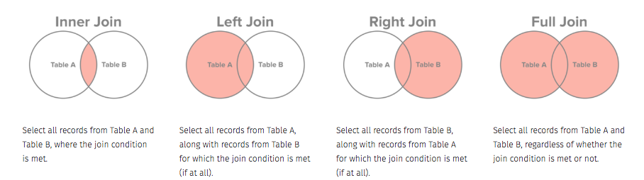
We mentioned earlier that there are several kinds of ways we can join data. The different kinds of joins are described below.

Let’s look at these joins with an example. We have two simulated datasets looking at DOS real estate allocation and staffing. We will look at how much area on average each bureau has given the number of employees

staffing_data <- import('data/Staffing_by_Bureau.csv') %>% as_tibble()
real_estate <- import('data/DoS_Real_Estate_Allocation.csv') %>% as_tibble()
real_estate

## # A tibble: 666 x 4
##    Building Bureau               Location  Size
##    <chr>    <chr>                   <int> <int>
##  1 HST      Administration (A)       4779   640
##  2 SA2      Administration (A)       4801  1090
##  3 HST      Administration (A)       5109  1040
##  4 HST      Administration (A)       3717  1620
##  5 SA4      Administration (A)       3940  1390
##  6 HST      Administration (A)       3661  1480
##  7 HST      Administration (A)       3374  1770
##  8 HST      Administration (A)       3387  1940
##  9 SA10     African Affairs (AF)     2605   640
## 10 HST      African Affairs (AF)     3573   720
## # … with 656 more rows

staffing_data

## # A tibble: 10,000 x 6
##    Bureau                      Gender Grade Title    Name      YearsService
##    <chr>                       <chr>  <chr> <chr>    <chr>            <int>
##  1 Protocol (S/CPR)            female FS1   Manager  Cathy Ca…           13
##  2 Administration (A)          male   GS-9  Team Me… Jeffery …           13
##  3 Intelligence and Research … male   FS-6  Analyst  Max Green           11
##  4 Mission to the United Nati… male   FS-3  Manager  Donald A…            7
##  5 Foreign Missions (OFM)      male   FS-6  Team Me… Thomas L…           22
##  6 International Narcotics an… male   GS-8  Team Me… Joseph A…           12
##  7 Administration (A)          male   GS-12 Analyst  Michael …            6
##  8 Intelligence and Research … male   FS-5  Team Me… Jesus Sh…            2
##  9 Science & Technology Advis… male   N/A   Manager  Lawrence…           19
## 10 Administration (A)          female FS-8  Team Me… Jennie C…           17
## # … with 9,990 more rows

The strategy is going to be to do a grouped summary of the staffing data to see how many people are in each Bureau, and then join that with the real estate data to compute the average area per employee by Bureau.

staff_summary <- staffing_data %>% 
  group_by(Bureau) %>% 
  tally(name = 'Pop')
realestate_summary <- real_estate %>% 
  group_by(Bureau) %>% summarize(Size = sum(Size))
realestate_summary %>% left_join(staff_summary) %>% 
  mutate(unit_area = Size/Pop) %>% 
  arrange(unit_area)

## Joining, by = "Bureau"

## # A tibble: 54 x 4
##    Bureau                                              Size   Pop unit_area
##    <chr>                                              <int> <int>     <dbl>
##  1 Global Youth Issues (GYI)                           2090   345      6.06
##  2 Policy Planning Staff (S/P)                         2420   240     10.1 
##  3 Science & Technology Adviser (STAS)                 4240   305     13.9 
##  4 Foreign Missions (OFM)                              4420   311     14.2 
##  5 Trafficking in Persons (TIP)                        5150   247     20.9 
##  6 Medical Services (MED)                              6760   308     21.9 
##  7 Protocol (S/CPR)                                    7730   327     23.6 
##  8 Administration (A)                                 10970   454     24.2 
##  9 Oceans and International Environmental and Scient…  8420   330     25.5 
## 10 Energy Resources (ENR)                             10890   369     29.5 
## # … with 44 more rows