Chapter 4 Pandas

4.1 Introduction

pandas is the Python Data Analysis package. It allows for data ingestion, transformation and cleaning, and creates objects that can then be passed on to analytic packages like statsmodels and scikit-learn for modeling and packages like matplotlib, seaborn, and plotly for visualization.

pandas is built on top of numpy, so many numpy functions are commonly used in manipulating pandas objects.

pandas is a pretty extensive package, and we’ll only be able to cover some of its features. For more details, there is free online documentation at pandas.pydata.org. You can also look at the book “Python for Data Analysis (2nd edition)” by Wes McKinney, the original developer of the pandas package, for more details.

4.2 Starting pandas

As with any Python module, you have to “activate” pandas by using import. The “standard” alias for pandas is pd. We will also import numpy, since pandas uses some numpy functions in the workflows.

import numpy as np
import pandas as pd

4.3 Data import and export

Most data sets you will work with are set up in tables, so are rectangular in shape. Think Excel spreadsheets. In pandas the structure that will hold this kind of data is a DataFrame. We can read external data into a DataFrame using one of many read_* functions. We can also write from a DataFrame to a variety of formats using to_* functions. The most common of these are listed below:

Format type	Description	reader	writer
text	CSV	read_csv	to_csv
	Excel	read_excel	to_excel
text	JSON	read_json	to_json
binary	Feather	read_feather	to_feather
binary	SAS	read_sas
SQL	SQL	read_sql	to_sql

We’ll start by reading in the mtcars dataset stored as a CSV file

pd.read_csv('data/mtcars.csv')

                   make   mpg  cyl   disp   hp  ...   qsec  vs  am  gear  carb
0             Mazda RX4  21.0    6  160.0  110  ...  16.46   0   1     4     4
1         Mazda RX4 Wag  21.0    6  160.0  110  ...  17.02   0   1     4     4
2            Datsun 710  22.8    4  108.0   93  ...  18.61   1   1     4     1
3        Hornet 4 Drive  21.4    6  258.0  110  ...  19.44   1   0     3     1
4     Hornet Sportabout  18.7    8  360.0  175  ...  17.02   0   0     3     2
5               Valiant  18.1    6  225.0  105  ...  20.22   1   0     3     1
6            Duster 360  14.3    8  360.0  245  ...  15.84   0   0     3     4
7             Merc 240D  24.4    4  146.7   62  ...  20.00   1   0     4     2
8              Merc 230  22.8    4  140.8   95  ...  22.90   1   0     4     2
9              Merc 280  19.2    6  167.6  123  ...  18.30   1   0     4     4
10            Merc 280C  17.8    6  167.6  123  ...  18.90   1   0     4     4
11           Merc 450SE  16.4    8  275.8  180  ...  17.40   0   0     3     3
12           Merc 450SL  17.3    8  275.8  180  ...  17.60   0   0     3     3
13          Merc 450SLC  15.2    8  275.8  180  ...  18.00   0   0     3     3
14   Cadillac Fleetwood  10.4    8  472.0  205  ...  17.98   0   0     3     4
15  Lincoln Continental  10.4    8  460.0  215  ...  17.82   0   0     3     4
16    Chrysler Imperial  14.7    8  440.0  230  ...  17.42   0   0     3     4
17             Fiat 128  32.4    4   78.7   66  ...  19.47   1   1     4     1
18          Honda Civic  30.4    4   75.7   52  ...  18.52   1   1     4     2
19       Toyota Corolla  33.9    4   71.1   65  ...  19.90   1   1     4     1
20        Toyota Corona  21.5    4  120.1   97  ...  20.01   1   0     3     1
21     Dodge Challenger  15.5    8  318.0  150  ...  16.87   0   0     3     2
22          AMC Javelin  15.2    8  304.0  150  ...  17.30   0   0     3     2
23           Camaro Z28  13.3    8  350.0  245  ...  15.41   0   0     3     4
24     Pontiac Firebird  19.2    8  400.0  175  ...  17.05   0   0     3     2
25            Fiat X1-9  27.3    4   79.0   66  ...  18.90   1   1     4     1
26        Porsche 914-2  26.0    4  120.3   91  ...  16.70   0   1     5     2
27         Lotus Europa  30.4    4   95.1  113  ...  16.90   1   1     5     2
28       Ford Pantera L  15.8    8  351.0  264  ...  14.50   0   1     5     4
29         Ferrari Dino  19.7    6  145.0  175  ...  15.50   0   1     5     6
30        Maserati Bora  15.0    8  301.0  335  ...  14.60   0   1     5     8
31           Volvo 142E  21.4    4  121.0  109  ...  18.60   1   1     4     2

[32 rows x 12 columns]

This just prints out the data, but then it’s lost. To use this data, we have to give it a name, so it’s stored in Python’s memory

mtcars = pd.read_csv('data/mtcars.csv')

One of the big differences between a spreadsheet program and a programming language from the data science perspective is that you have to load data into the programming language. It’s not “just there” like Excel. This is a good thing, since it allows the common functionality of the programming language to work across multiple data sets, and also keeps the original data set pristine. Excel users can run into problems and corrupt their data if they are not careful.

If we wanted to write this data set back out into an Excel file, say, we could do

mtcars.to_excel('data/mtcars.xlsx')

You may get an error if you don’t have the openpyxl package installed. You can easily install it from the Anaconda prompt using conda install openpyxl and following the prompts.

4.4 Exploring a data set

We would like to get some idea about this data set. There are a bunch of functions linked to the DataFrame object that help us in this. First we will use head to see the first 8 rows of this data set

mtcars.head(8)

                make   mpg  cyl   disp   hp  ...   qsec  vs  am  gear  carb
0          Mazda RX4  21.0    6  160.0  110  ...  16.46   0   1     4     4
1      Mazda RX4 Wag  21.0    6  160.0  110  ...  17.02   0   1     4     4
2         Datsun 710  22.8    4  108.0   93  ...  18.61   1   1     4     1
3     Hornet 4 Drive  21.4    6  258.0  110  ...  19.44   1   0     3     1
4  Hornet Sportabout  18.7    8  360.0  175  ...  17.02   0   0     3     2
5            Valiant  18.1    6  225.0  105  ...  20.22   1   0     3     1
6         Duster 360  14.3    8  360.0  245  ...  15.84   0   0     3     4
7          Merc 240D  24.4    4  146.7   62  ...  20.00   1   0     4     2

[8 rows x 12 columns]

This is our first look into this data. We notice a few things. Each column has a name, and each row has an index, starting at 0.

If you’re interested in the last N rows, there is a corresponding tail function

Let’s look at the data types of each of the columns

mtcars.dtypes

make     object
mpg     float64
cyl       int64
disp    float64
hp        int64
drat    float64
wt      float64
qsec    float64
vs        int64
am        int64
gear      int64
carb      int64
dtype: object

This tells us that some of the variables, like mpg and disp, are floating point (decimal) numbers, several are integers, and make is an “object”. The dtypes function borrows from numpy, where there isn’t really a type for character or categorical variables. So most often, when you see “object” in the output of dtypes, you think it’s a character or categorical variable.

We can also look at the data structure in a bit more detail.

mtcars.info()

<class 'pandas.core.frame.DataFrame'>
RangeIndex: 32 entries, 0 to 31
Data columns (total 12 columns):
 #   Column  Non-Null Count  Dtype  
---  ------  --------------  -----  
 0   make    32 non-null     object 
 1   mpg     32 non-null     float64
 2   cyl     32 non-null     int64  
 3   disp    32 non-null     float64
 4   hp      32 non-null     int64  
 5   drat    32 non-null     float64
 6   wt      32 non-null     float64
 7   qsec    32 non-null     float64
 8   vs      32 non-null     int64  
 9   am      32 non-null     int64  
 10  gear    32 non-null     int64  
 11  carb    32 non-null     int64  
dtypes: float64(5), int64(6), object(1)
memory usage: 3.1+ KB

This tells us that this is indeed a DataFrame, wth 12 columns, each with 32 valid observations. Each row has an index value ranging from 0 to 11. We also get the approximate size of this object in memory.

You can also quickly find the number of rows and columns of a data set by using shape, which is borrowed from numpy.

mtcars.shape

(32, 12)

More generally, we can get a summary of each variable using the describe function

mtcars.describe()

             mpg        cyl        disp  ...         am       gear     carb
count  32.000000  32.000000   32.000000  ...  32.000000  32.000000  32.0000
mean   20.090625   6.187500  230.721875  ...   0.406250   3.687500   2.8125
std     6.026948   1.785922  123.938694  ...   0.498991   0.737804   1.6152
min    10.400000   4.000000   71.100000  ...   0.000000   3.000000   1.0000
25%    15.425000   4.000000  120.825000  ...   0.000000   3.000000   2.0000
50%    19.200000   6.000000  196.300000  ...   0.000000   4.000000   2.0000
75%    22.800000   8.000000  326.000000  ...   1.000000   4.000000   4.0000
max    33.900000   8.000000  472.000000  ...   1.000000   5.000000   8.0000

[8 rows x 11 columns]

These are usually the first steps in exploring the data.

4.5 Data structures and types

pandas has two main data types: Series and DataFrame. These are analogous to vectors and matrices, in that a Series is 1-dimensional while a DataFrame is 2-dimensional.

4.5.1 pandas.Series

The Series object holds data from a single input variable, and is required, much like numpy arrays, to be homogeneous in type. You can create Series objects from lists or numpy arrays quite easily

s = pd.Series([1,3,5,np.nan, 9, 13])
s

0     1.0
1     3.0
2     5.0
3     NaN
4     9.0
5    13.0
dtype: float64

s2 = pd.Series(np.arange(1,20))
s2

0      1
1      2
2      3
3      4
4      5
5      6
6      7
7      8
8      9
9     10
10    11
11    12
12    13
13    14
14    15
15    16
16    17
17    18
18    19
dtype: int64

You can access elements of a Series much like a dict

s2[4]

There is no requirement that the index of a Series has to be numeric. It can be any kind of scalar object

s3 = pd.Series(np.random.normal(0,1, (5,)), index = ['a','b','c','d','e'])
s3

a   -0.283473
b    0.157530
c    1.051739
d    0.859905
e    1.178951
dtype: float64

s3['d']

0.859904696094078

s3['a':'d']

a   -0.283473
b    0.157530
c    1.051739
d    0.859905
dtype: float64

Well, slicing worked, but it gave us something different than expected. It gave us both the start and end of the slice, which is unlike what we’ve encountered so far!!

It turns out that in pandas, slicing by index actually does this. It is a discrepancy from numpy and Python in general that we have to be careful about.

You can extract the actual values into a numpy array

s3.to_numpy()

array([-0.28347282,  0.1575304 ,  1.05173885,  0.8599047 ,  1.17895111])

In fact, you’ll see that much of pandas’ structures are build on top of numpy arrays. This is a good thing, since you can take advantage of the powerful numpy functions that are built for fast, efficient scientific computing.

Making the point about slicing again,

s3.to_numpy()[0:3]

array([-0.28347282,  0.1575304 ,  1.05173885])

This is different from index-based slicing done earlier.

4.5.2 pandas.DataFrame

The DataFrame object holds a rectangular data set. Each column of a DataFrame is a Series object. This means that each column of a DataFrame must be comprised of data of the same type, but different columns can hold data of different types. This structure is extremely useful in practical data science. The invention of this structure was, in my opinion, transformative in making Python an effective data science tool.

4.5.2.1 Creating a DataFrame

The DataFrame can be created by importing data, as we saw in the previous section. It can also be created by a few methods within Python.

First, it can be created from a 2-dimensional numpy array.

rng = np.random.RandomState(25)
d1 = pd.DataFrame(rng.normal(0,1, (4,5)))
d1

          0         1         2         3         4
0  0.228273  1.026890 -0.839585 -0.591182 -0.956888
1 -0.222326 -0.619915  1.837905 -2.053231  0.868583
2 -0.920734 -0.232312  2.152957 -1.334661  0.076380
3 -1.246089  1.202272 -1.049942  1.056610 -0.419678

You will notice that it creates default column names, that are merely the column number, starting from 0. We can also create the column names and row index (similar to the Series index we saw earlier) directly during creation.

d2 = pd.DataFrame(rng.normal(0,1, (4, 5)), 
                  columns = ['A','B','C','D','E'], 
                  index = ['a','b','c','d'])
d2

          A         B         C         D         E
a  2.294842 -2.594487  2.822756  0.680889 -1.577693
b -1.976254  0.533340 -0.290870 -0.513520  1.982626
c  0.226001 -1.839905  1.607671  0.388292  0.399732
d  0.405477  0.217002 -0.633439  0.246622 -1.939546

We could also create a DataFrame from a list of lists, as long as things line up, just as we showed for numpy arrays. However, to me, other ways, including the dict method below, make more sense.

We can change the column names (which can be extracted and replaced with the columns attribute) and the index values (using the index attribute).

d2.columns

Index(['A', 'B', 'C', 'D', 'E'], dtype='object')

d2.columns = pd.Index(['V'+str(i) for i in range(1,6)]) # Index creates the right objects for both column names and row names, which can be extracted and changed with the `index` attribute
d2

         V1        V2        V3        V4        V5
a  2.294842 -2.594487  2.822756  0.680889 -1.577693
b -1.976254  0.533340 -0.290870 -0.513520  1.982626
c  0.226001 -1.839905  1.607671  0.388292  0.399732
d  0.405477  0.217002 -0.633439  0.246622 -1.939546

Exercise: Can you explain what I did in the list comprehension above? The key points are understanding str and how I constructed the range.

d2.index = ['o1','o2','o3','o4']
d2

          V1        V2        V3        V4        V5
o1  2.294842 -2.594487  2.822756  0.680889 -1.577693
o2 -1.976254  0.533340 -0.290870 -0.513520  1.982626
o3  0.226001 -1.839905  1.607671  0.388292  0.399732
o4  0.405477  0.217002 -0.633439  0.246622 -1.939546

You can also extract data from a homogeneous DataFrame to a numpy array

d1.to_numpy()

array([[ 0.22827309,  1.0268903 , -0.83958485, -0.59118152, -0.9568883 ],
       [-0.22232569, -0.61991511,  1.83790458, -2.05323076,  0.86858305],
       [-0.92073444, -0.23231186,  2.1529569 , -1.33466147,  0.07637965],
       [-1.24608928,  1.20227231, -1.04994158,  1.05661011, -0.41967767]])

It turns out that you can use to_numpy for a non-homogeneous DataFrame as well. numpy just makes it homogeneous by assigning each column the data type object. This also limits what you can do in numpy with the array and may require changing data types using the astype function. There is some more detail about the object data type in the Python Tools for Data Science (notebook, PDF) document.

The other easy way to create a DataFrame is from a dict object, where each component object is either a list or a numpy array, and is homogeneous in type. One exception is if a component is of size 1; then it is repeated to meet the needs of the DataFrame’s dimensions

df = pd.DataFrame({
    'A':3.,
    'B':rng.random_sample(5),
    'C': pd.Timestamp('20200512'),
    'D': np.array([6] * 5),
    'E': pd.Categorical(['yes','no','no','yes','no']),
    'F': 'NIH'})
df

     A         B          C  D    E    F
0  3.0  0.958092 2020-05-12  6  yes  NIH
1  3.0  0.883201 2020-05-12  6   no  NIH
2  3.0  0.295432 2020-05-12  6   no  NIH
3  3.0  0.512376 2020-05-12  6  yes  NIH
4  3.0  0.088702 2020-05-12  6   no  NIH

df.info()

<class 'pandas.core.frame.DataFrame'>
RangeIndex: 5 entries, 0 to 4
Data columns (total 6 columns):
 #   Column  Non-Null Count  Dtype         
---  ------  --------------  -----         
 0   A       5 non-null      float64       
 1   B       5 non-null      float64       
 2   C       5 non-null      datetime64[ns]
 3   D       5 non-null      int64         
 4   E       5 non-null      category      
 5   F       5 non-null      object        
dtypes: category(1), datetime64[ns](1), float64(2), int64(1), object(1)
memory usage: 429.0+ bytes

We note that C is a date object, E is a category object, and F is a text/string object. pandas has excellent time series capabilities (having origins in FinTech), and the TimeStamp function creates datetime objects which can be queried and manipulated in Python. We’ll describe category data in the next section.

You can also create a DataFrame where each column is composed of composite objects, like lists and dicts, as well. This might have limited value in some settings, but may be useful in others. In particular, this allows capabilities like the list-column construct in R tibbles. For example,

pd.DataFrame({'list' :[[1,2],[3,4],[5,6]],
             'tuple' : [('a','b'), ('c','d'), ('e','f')],
              'set' : [{'A','B','C'}, {'D','E'}, {'F'}], 
            'dicts' : [{'A': [1,2,3]}, {'B':[5,6,8]}, {'C': [3,9]}]})

     list   tuple        set             dicts
0  [1, 2]  (a, b)  {B, A, C}  {'A': [1, 2, 3]}
1  [3, 4]  (c, d)     {E, D}  {'B': [5, 6, 8]}
2  [5, 6]  (e, f)        {F}     {'C': [3, 9]}

4.5.2.2 Working with a DataFrame

You can extract particular columns of a DataFrame by name

df['E']

0    yes
1     no
2     no
3    yes
4     no
Name: E, dtype: category
Categories (2, object): [no, yes]

df['B']

0    0.958092
1    0.883201
2    0.295432
3    0.512376
4    0.088702
Name: B, dtype: float64

There is also a shortcut for accessing single columns, using Python’s dot (.) notation.

df.B

0    0.958092
1    0.883201
2    0.295432
3    0.512376
4    0.088702
Name: B, dtype: float64

This notation can be more convenient if we need to perform operations on a single column. If we want to extract multiple columns, this notation will not work. Also, if we want to create new columns or replace existing columns, we need to use the array notation with the column name in quotes.

Let’s look at slicing a DataFrame

4.5.2.3 Extracting rows and columns

There are two extractor functions in pandas:

loc extracts by label (index label, column label, slice of labels, etc.
iloc extracts by index (integers, slice objects, etc.

df2 = pd.DataFrame(rng.randint(0,10, (5,4)), 
                  index = ['a','b','c','d','e'],
                  columns = ['one','two','three','four'])
df2

   one  two  three  four
a    5    3      2     8
b    9    3      0     5
c    8    4      3     3
d    5    2      7     1
e    6    7      8     7

First, let’s see what naively slicing this DataFrame does.

df2['one']

a    5
b    9
c    8
d    5
e    6
Name: one, dtype: int64

Ok, that works. It grabs one column from the dataset. How about the dot notation?

df2.one

a    5
b    9
c    8
d    5
e    6
Name: one, dtype: int64

Let’s see what this produces.

type(df2.one)

<class 'pandas.core.series.Series'>

So this is a series, so we can potentially do slicing of this series.

df2.one['b']

df2.one['b':'d']

b    9
c    8
d    5
Name: one, dtype: int64

df2.one[:3]

a    5
b    9
c    8
Name: one, dtype: int64

Ok, so we have all the Series slicing available. The problem here is in semantics, in that we are grabbing one column and then slicing the rows. That doesn’t quite work with our sense that a DataFrame is a rectangle with rows and columns, and we tend to think of rows, then columns.

Let’s see if we can do column slicing with this.

df2[:'two']

   one  two  three  four
a    5    3      2     8
b    9    3      0     5
c    8    4      3     3
d    5    2      7     1
e    6    7      8     7

That’s not what we want, of course. It’s giving back the entire data frame. We’ll come back to this.

df2[['one','three']]

   one  three
a    5      2
b    9      0
c    8      3
d    5      7
e    6      8

That works correctly though. We can give a list of column names. Ok.

How about row slices?

#df2['a'] # Doesn't work
df2['a':'c']

   one  two  three  four
a    5    3      2     8
b    9    3      0     5
c    8    4      3     3

Ok, that works. It slices rows, but includes the largest index, like a Series but unlike numpy arrays.

df2[0:2]

   one  two  three  four
a    5    3      2     8
b    9    3      0     5

Slices by location work too, but use the numpy slicing rules.

This entire extraction method becomes confusing. Let’s simplify things for this, and then move on to more consistent ways to extract elements of a DataFrame. Let’s agree on two things. If we’re going the direct extraction route,

We will extract single columns of a DataFrame with [] or ., i.e., df2['one'] or df2.one
We will extract slices of rows of a DataFrame using location only, i.e., df2[:3].

For everything else, we’ll use two functions, loc and iloc.

loc extracts elements like a matrix, using index and columns
iloc extracts elements like a matrix, using location

df2.loc[:,'one':'three']

   one  two  three
a    5    3      2
b    9    3      0
c    8    4      3
d    5    2      7
e    6    7      8

df2.loc['a':'d',:]

   one  two  three  four
a    5    3      2     8
b    9    3      0     5
c    8    4      3     3
d    5    2      7     1

df2.loc['b', 'three']

So loc works just like a matrix, but with pandas slicing rules (include largest index)

df2.iloc[:,1:4]

   two  three  four
a    3      2     8
b    3      0     5
c    4      3     3
d    2      7     1
e    7      8     7

df2.iloc[1:3,:]

   one  two  three  four
b    9    3      0     5
c    8    4      3     3

df2.iloc[1:3, 1:4]

   two  three  four
b    3      0     5
c    4      3     3

iloc slices like a matrix, but uses numpy slicing conventions (does not include highest index)

If we want to extract a single element from a dataset, there are two functions available, iat and at, with behavior corresponding to iloc and loc, respectively.

df2.iat[2,3]

df2.at['b','three']

4.5.2.4 Boolean selection

We can also use tests to extract data from a DataFrame. For example, we can extract only rows where column labeled one is greater than 3.

df2[df2.one > 3]

   one  two  three  four
a    5    3      2     8
b    9    3      0     5
c    8    4      3     3
d    5    2      7     1
e    6    7      8     7

We can also do composite tests. Here we ask for rows where one is greater than 3 and three is less than 9

df2[(df2.one > 3) & (df2.three < 9)]

   one  two  three  four
a    5    3      2     8
b    9    3      0     5
c    8    4      3     3
d    5    2      7     1
e    6    7      8     7

4.5.2.5 `query`

DataFrame’s have a query method allowing selection using a Python expression

n = 10
df = pd.DataFrame(np.random.rand(n, 3), columns = list('abc'))
df

          a         b         c
0  0.824319  0.095623  0.459736
1  0.200426  0.302179  0.534959
2  0.381447  0.775250  0.654027
3  0.482755  0.512036  0.763493
4  0.679697  0.972007  0.946838
5  0.111028  0.909652  0.136886
6  0.817464  0.499767  0.769067
7  0.921952  0.481407  0.479161
8  0.626052  0.484680  0.518859
9  0.497046  0.045412  0.324195

df[(df.a < df.b) & (df.b < df.c)]

          a         b         c
1  0.200426  0.302179  0.534959
3  0.482755  0.512036  0.763493

We can equivalently write this query as

df.query('(a < b) & (b < c)')

          a         b         c
1  0.200426  0.302179  0.534959
3  0.482755  0.512036  0.763493

4.5.2.6 Replacing values in a DataFrame

We can replace values within a DataFrame either by position or using a query.

df2

   one  two  three  four
a    5    3      2     8
b    9    3      0     5
c    8    4      3     3
d    5    2      7     1
e    6    7      8     7

df2['one'] = [2,5,2,5,2]
df2

   one  two  three  four
a    2    3      2     8
b    5    3      0     5
c    2    4      3     3
d    5    2      7     1
e    2    7      8     7

df2.iat[2,3] = -9 # missing value
df2

   one  two  three  four
a    2    3      2     8
b    5    3      0     5
c    2    4      3    -9
d    5    2      7     1
e    2    7      8     7

Let’s now replace values using replace which is more flexible.

df2.replace(0, -9) # replace 0 with -9

   one  two  three  four
a    2    3      2     8
b    5    3     -9     5
c    2    4      3    -9
d    5    2      7     1
e    2    7      8     7

df2.replace({2: 2.5, 8: 6.5}) # multiple replacements

   one  two  three  four
a  2.5  3.0    2.5   6.5
b  5.0  3.0    0.0   5.0
c  2.5  4.0    3.0  -9.0
d  5.0  2.5    7.0   1.0
e  2.5  7.0    6.5   7.0

df2.replace({'one': {5: 500}, 'three': {0: -9, 8: 800}}) 
# different replacements in different columns

   one  two  three  four
a    2    3      2     8
b  500    3     -9     5
c    2    4      3    -9
d  500    2      7     1
e    2    7    800     7

See more examples in the documentation

4.5.3 Categorical data

pandas provides a Categorical function and a category object type to Python. This type is analogous to the factor data type in R. It is meant to address categorical or discrete variables, where we need to use them in analyses. Categorical variables typically take on a small number of unique values, like gender, blood type, country of origin, race, etc.

You can create categorical Series in a couple of ways:

s = pd.Series(['a','b','c'], dtype='category')

df = pd.DataFrame({
    'A':3.,
    'B':rng.random_sample(5),
    'C': pd.Timestamp('20200512'),
    'D': np.array([6] * 5),
    'E': pd.Categorical(['yes','no','no','yes','no']),
    'F': 'NIH'})
df['F'].astype('category')

0    NIH
1    NIH
2    NIH
3    NIH
4    NIH
Name: F, dtype: category
Categories (1, object): [NIH]

You can also create DataFrame’s where each column is categorical

df = pd.DataFrame({'A': list('abcd'), 'B': list('bdca')})
df_cat = df.astype('category')
df_cat.dtypes

A    category
B    category
dtype: object

You can explore categorical data in a variety of ways

df_cat['A'].describe()

count     4
unique    4
top       d
freq      1
Name: A, dtype: object

df['A'].value_counts()

d    1
b    1
a    1
c    1
Name: A, dtype: int64

One issue with categories is that, if a particular level of a category is not seen before, it can create an error. So you can pre-specify the categories you expect

df_cat['B'] = pd.Categorical(list('aabb'), categories = ['a','b','c','d'])
df_cat['B'].value_counts()

b    2
a    2
d    0
c    0
Name: B, dtype: int64

4.5.3.1 Re-organizing categories

In categorical data, there is often the concept of a “first” or “reference” category, and an ordering of categories. This tends to be important in both visualization as well as in regression modeling. Both aspects of a category can be addressed using the reorder_categories function.

In our earlier example, we can see that the A variable has 4 categories, with the “first” category being “a”.

df_cat.A

0    a
1    b
2    c
3    d
Name: A, dtype: category
Categories (4, object): [a, b, c, d]

Suppose we want to change this ordering to the reverse ordering, where “d” is the “first” category, and then it goes in reverse order.

df_cat['A'] = df_cat.A.cat.reorder_categories(['d','c','b','a'])
df_cat.A

0    a
1    b
2    c
3    d
Name: A, dtype: category
Categories (4, object): [d, c, b, a]

4.5.4 Missing data

Both numpy and pandas allow for missing values, which are a reality in data science. The missing values are coded as np.nan. Let’s create some data and force some missing values

df = pd.DataFrame(np.random.randn(5, 3), index = ['a','c','e', 'f','g'], columns = ['one','two','three']) # pre-specify index and column names
df['four'] = 20 # add a column named "four", which will all be 20
df['five'] = df['one'] > 0
df

        one       two     three  four   five
a -0.706987 -0.821679  1.441257    20  False
c  1.297128  0.501395  0.572570    20   True
e -0.761507  1.469939  0.400255    20  False
f -0.910821  0.449404  0.588879    20  False
g -0.718350 -0.364237  1.793386    20  False

df2 = df.reindex(['a','b','c','d','e','f','g'])
df2.style.applymap(lambda x: 'background-color:yellow', subset = pd.IndexSlice[['b','d'],:])

<pandas.io.formats.style.Styler object at 0x11cbd6040>

The code above is creating new blank rows based on the new index values, some of which are present in the existing data and some of which are missing.

We can create masks of the data indicating where missing values reside in a data set.

df2.isna()

     one    two  three   four   five
a  False  False  False  False  False
b   True   True   True   True   True
c  False  False  False  False  False
d   True   True   True   True   True
e  False  False  False  False  False
f  False  False  False  False  False
g  False  False  False  False  False

df2['one'].notna()

a     True
b    False
c     True
d    False
e     True
f     True
g     True
Name: one, dtype: bool

We can obtain complete data by dropping any row that has any missing value. This is called complete case analysis, and you should be very careful using it. It is only valid if we belive that the missingness is missing at random, and not related to some characteristic of the data or the data gathering process.

df2.dropna(how='any')

        one       two     three  four   five
a -0.706987 -0.821679  1.441257  20.0  False
c  1.297128  0.501395  0.572570  20.0   True
e -0.761507  1.469939  0.400255  20.0  False
f -0.910821  0.449404  0.588879  20.0  False
g -0.718350 -0.364237  1.793386  20.0  False

You can also fill in, or impute, missing values. This can be done using a single value..

out1 = df2.fillna(value = 5)

out1.style.applymap(lambda x: 'background-color:yellow', subset = pd.IndexSlice[['b','d'],:])

<pandas.io.formats.style.Styler object at 0x11cf5fca0>

or a computed value like a column mean

df3 = df2.copy()
df3 = df3.select_dtypes(exclude=[object])   # remove non-numeric columns
out2 = df3.fillna(df3.mean())  # df3.mean() computes column-wise means

out2.style.applymap(lambda x: 'background-color:yellow', subset = pd.IndexSlice[['b','d'],:])

<pandas.io.formats.style.Styler object at 0x11cf830d0>

You can also impute based on the principle of last value carried forward which is common in time series. This means that the missing value is imputed with the previous recorded value.

out3 = df2.fillna(method = 'ffill') # Fill forward

out3.style.applymap(lambda x: 'background-color:yellow', subset = pd.IndexSlice[['b','d'],:])

<pandas.io.formats.style.Styler object at 0x11cbeca60>

out4 = df2.fillna(method = 'bfill') # Fill backward

out4.style.applymap(lambda x: 'background-color:yellow', subset = pd.IndexSlice[['b','d'],:])

<pandas.io.formats.style.Styler object at 0x11cbd6ca0>

4.6 Data transformation

4.6.1 Arithmetic operations

If you have a Series or DataFrame that is all numeric, you can add or multiply single numbers to all the elements together.

A = pd.DataFrame(np.random.randn(4,5))
print(A)

          0         1         2         3         4
0  0.243690  1.076332  0.950349  1.373858  0.868005
1  2.712568  1.046159 -2.044472 -0.630508  0.945787
2  0.413522  1.938513 -0.195251  0.350383  1.381913
3 -0.927886 -1.882394 -2.163616 -0.142430  1.091522

print(A + 6)

          0         1         2         3         4
0  6.243690  7.076332  6.950349  7.373858  6.868005
1  8.712568  7.046159  3.955528  5.369492  6.945787
2  6.413522  7.938513  5.804749  6.350383  7.381913
3  5.072114  4.117606  3.836384  5.857570  7.091522

print(A * -10)

           0          1          2          3          4
0  -2.436896 -10.763319  -9.503492 -13.738582  -8.680051
1 -27.125677 -10.461590  20.444719   6.305081  -9.457871
2  -4.135220 -19.385126   1.952507  -3.503830 -13.819127
3   9.278864  18.823936  21.636155   1.424302 -10.915223

If you have two compatible (same dimension) numeric DataFrames, you can add, subtract, multiply and divide elementwise

B = pd.DataFrame(np.random.randn(4,5) + 4)
print(A + B)

          0         1         2         3         4
0  4.018707  5.687454  3.580436  6.782426  5.120555
1  5.253674  6.124992  1.169963  2.695430  5.307602
2  4.217585  5.948985  4.620141  4.040466  4.649786
3  3.890115  2.221573  1.245353  5.396740  5.127738

print(A * B)

          0         1         2         3         4
0  0.919932  4.963098  2.499501  7.430605  3.691235
1  6.892923  5.313267 -6.571821 -2.097031  4.125348
2  1.573064  7.774351 -0.940208  1.292943  4.515915
3 -4.470558 -7.725281 -7.375697 -0.788945  4.405619

If you have a Series with the same number of elements as the number of columns of a DataFrame, you can do arithmetic operations, with each element of the Series acting upon each column of the DataFrame

c = pd.Series([1,2,3,4,5])
print(A + c)

          0         1         2         3         4
0  1.243690  3.076332  3.950349  5.373858  5.868005
1  3.712568  3.046159  0.955528  3.369492  5.945787
2  1.413522  3.938513  2.804749  4.350383  6.381913
3  0.072114  0.117606  0.836384  3.857570  6.091522

print(A * c)

          0         1         2         3         4
0  0.243690  2.152664  2.851048  5.495433  4.340025
1  2.712568  2.092318 -6.133416 -2.522032  4.728935
2  0.413522  3.877025 -0.585752  1.401532  6.909563
3 -0.927886 -3.764787 -6.490847 -0.569721  5.457611

This idea can be used to standardize a dataset, i.e. make each column have mean 0 and standard deviation 1.

means = A.mean(axis=0)
stds = A.std(axis = 0)

(A - means)/stds

          0         1         2         3         4
0 -0.240828  0.318354  1.202702  1.326047 -0.899601
1  1.380224  0.300287 -0.783339 -1.013572 -0.556263
2 -0.129317  0.834602  0.442988  0.131384  1.368838
3 -1.010079 -1.453244 -0.862351 -0.443858  0.087026

4.6.2 Concatenation of data sets

Let’s create some example data sets

df1 = pd.DataFrame({'A': ['a'+str(i) for i in range(4)],
    'B': ['b'+str(i) for i in range(4)],
    'C': ['c'+str(i) for i in range(4)],
    'D': ['d'+str(i) for i in range(4)]})

df2 =  pd.DataFrame({'A': ['a'+str(i) for i in range(4,8)],
    'B': ['b'+str(i) for i in range(4,8)],
    'C': ['c'+str(i) for i in range(4,8)],
    'D': ['d'+str(i) for i in range(4,8)]})
df3 =  pd.DataFrame({'A': ['a'+str(i) for i in range(8,12)],
    'B': ['b'+str(i) for i in range(8,12)],
    'C': ['c'+str(i) for i in range(8,12)],
    'D': ['d'+str(i) for i in range(8,12)]})

We can concatenate these DataFrame objects by row

row_concatenate = pd.concat([df1, df2, df3])
print(row_concatenate)

     A    B    C    D
0   a0   b0   c0   d0
1   a1   b1   c1   d1
2   a2   b2   c2   d2
3   a3   b3   c3   d3
0   a4   b4   c4   d4
1   a5   b5   c5   d5
2   a6   b6   c6   d6
3   a7   b7   c7   d7
0   a8   b8   c8   d8
1   a9   b9   c9   d9
2  a10  b10  c10  d10
3  a11  b11  c11  d11

This stacks the dataframes together. They are literally stacked, as is evidenced by the index values being repeated.

This same exercise can be done by the append function

df1.append(df2).append(df3)

     A    B    C    D
0   a0   b0   c0   d0
1   a1   b1   c1   d1
2   a2   b2   c2   d2
3   a3   b3   c3   d3
0   a4   b4   c4   d4
1   a5   b5   c5   d5
2   a6   b6   c6   d6
3   a7   b7   c7   d7
0   a8   b8   c8   d8
1   a9   b9   c9   d9
2  a10  b10  c10  d10
3  a11  b11  c11  d11

Suppose we want to append a new row to df1. Lets create a new row.

new_row = pd.Series(['n1','n2','n3','n4'])
pd.concat([df1, new_row])

     A    B    C    D    0
0   a0   b0   c0   d0  NaN
1   a1   b1   c1   d1  NaN
2   a2   b2   c2   d2  NaN
3   a3   b3   c3   d3  NaN
0  NaN  NaN  NaN  NaN   n1
1  NaN  NaN  NaN  NaN   n2
2  NaN  NaN  NaN  NaN   n3
3  NaN  NaN  NaN  NaN   n4

That’s a lot of missing values. The issue is that the we don’t have column names in the new_row, and the indices are the same, so pandas tries to append it my making a new column. The solution is to make it a DataFrame.

new_row = pd.DataFrame([['n1','n2','n3','n4']], columns = ['A','B','C','D'])
print(new_row)

    A   B   C   D
0  n1  n2  n3  n4

pd.concat([df1, new_row])

    A   B   C   D
0  a0  b0  c0  d0
1  a1  b1  c1  d1
2  a2  b2  c2  d2
3  a3  b3  c3  d3
0  n1  n2  n3  n4

df1.append(new_row)

    A   B   C   D
0  a0  b0  c0  d0
1  a1  b1  c1  d1
2  a2  b2  c2  d2
3  a3  b3  c3  d3
0  n1  n2  n3  n4

4.6.2.1 Adding columns

pd.concat([df1,df2,df3], axis = 1)

    A   B   C   D   A   B   C   D    A    B    C    D
0  a0  b0  c0  d0  a4  b4  c4  d4   a8   b8   c8   d8
1  a1  b1  c1  d1  a5  b5  c5  d5   a9   b9   c9   d9
2  a2  b2  c2  d2  a6  b6  c6  d6  a10  b10  c10  d10
3  a3  b3  c3  d3  a7  b7  c7  d7  a11  b11  c11  d11

The option axis=1 ensures that concatenation happens by columns. The default value axis = 0 concatenates by rows.

Let’s play a little game. Let’s change the column names of df2 and df3 so they are not the same as df1.

df2.columns = ['E','F','G','H']
df3.columns = ['A','D','F','H']
pd.concat([df1,df2,df3])

     A    B    C    D    E    F    G    H
0   a0   b0   c0   d0  NaN  NaN  NaN  NaN
1   a1   b1   c1   d1  NaN  NaN  NaN  NaN
2   a2   b2   c2   d2  NaN  NaN  NaN  NaN
3   a3   b3   c3   d3  NaN  NaN  NaN  NaN
0  NaN  NaN  NaN  NaN   a4   b4   c4   d4
1  NaN  NaN  NaN  NaN   a5   b5   c5   d5
2  NaN  NaN  NaN  NaN   a6   b6   c6   d6
3  NaN  NaN  NaN  NaN   a7   b7   c7   d7
0   a8  NaN  NaN   b8  NaN   c8  NaN   d8
1   a9  NaN  NaN   b9  NaN   c9  NaN   d9
2  a10  NaN  NaN  b10  NaN  c10  NaN  d10
3  a11  NaN  NaN  b11  NaN  c11  NaN  d11

Now pandas ensures that all column names are represented in the new data frame, but with missing values where the row indices and column indices are mismatched. Some of this can be avoided by only joining on common columns. This is done using the join option ir concat. The default value is ’outer`, which is what you see. above

pd.concat([df1, df3], join = 'inner')

     A    D
0   a0   d0
1   a1   d1
2   a2   d2
3   a3   d3
0   a8   b8
1   a9   b9
2  a10  b10
3  a11  b11

You can do the same thing when joining by rows, using axis = 0 and join="inner" to only join on rows with matching indices. Reminder that the indices are just labels and happen to be the row numbers by default.

4.6.3 Merging data sets

For this section we’ll use a set of data from a survey, also used by Daniel Chen in “Pandas for Everyone”

person = pd.read_csv('data/survey_person.csv')
site = pd.read_csv('data/survey_site.csv')
survey = pd.read_csv('data/survey_survey.csv')
visited = pd.read_csv('data/survey_visited.csv')

print(person)

      ident   personal    family
0      dyer    William      Dyer
1        pb      Frank   Pabodie
2      lake   Anderson      Lake
3       roe  Valentina   Roerich
4  danforth      Frank  Danforth

print(site)

    name    lat    long
0   DR-1 -49.85 -128.57
1   DR-3 -47.15 -126.72
2  MSK-4 -48.87 -123.40

print(survey)

    taken person quant  reading
0     619   dyer   rad     9.82
1     619   dyer   sal     0.13
2     622   dyer   rad     7.80
3     622   dyer   sal     0.09
4     734     pb   rad     8.41
5     734   lake   sal     0.05
6     734     pb  temp   -21.50
7     735     pb   rad     7.22
8     735    NaN   sal     0.06
9     735    NaN  temp   -26.00
10    751     pb   rad     4.35
11    751     pb  temp   -18.50
12    751   lake   sal     0.10
13    752   lake   rad     2.19
14    752   lake   sal     0.09
15    752   lake  temp   -16.00
16    752    roe   sal    41.60
17    837   lake   rad     1.46
18    837   lake   sal     0.21
19    837    roe   sal    22.50
20    844    roe   rad    11.25

print(visited)

   ident   site       dated
0    619   DR-1  1927-02-08
1    622   DR-1  1927-02-10
2    734   DR-3  1939-01-07
3    735   DR-3  1930-01-12
4    751   DR-3  1930-02-26
5    752   DR-3         NaN
6    837  MSK-4  1932-01-14
7    844   DR-1  1932-03-22

There are basically four kinds of joins:

pandas	R	SQL	Description
left	left_join	left outer	keep all rows on left
right	right_join	right outer	keep all rows on right
outer	outer_join	full outer	keep all rows from both
inner	inner_join	inner	keep only rows with common keys

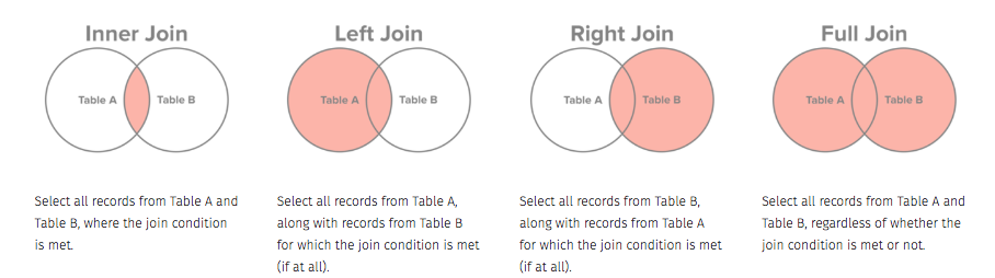
The terms left and right refer to which data set you call first and second respectively.

We start with an left join

s2v_merge = survey.merge(visited, left_on = 'taken',right_on = 'ident', how = 'left')

print(s2v_merge)

    taken person quant  reading  ident   site       dated
0     619   dyer   rad     9.82    619   DR-1  1927-02-08
1     619   dyer   sal     0.13    619   DR-1  1927-02-08
2     622   dyer   rad     7.80    622   DR-1  1927-02-10
3     622   dyer   sal     0.09    622   DR-1  1927-02-10
4     734     pb   rad     8.41    734   DR-3  1939-01-07
5     734   lake   sal     0.05    734   DR-3  1939-01-07
6     734     pb  temp   -21.50    734   DR-3  1939-01-07
7     735     pb   rad     7.22    735   DR-3  1930-01-12
8     735    NaN   sal     0.06    735   DR-3  1930-01-12
9     735    NaN  temp   -26.00    735   DR-3  1930-01-12
10    751     pb   rad     4.35    751   DR-3  1930-02-26
11    751     pb  temp   -18.50    751   DR-3  1930-02-26
12    751   lake   sal     0.10    751   DR-3  1930-02-26
13    752   lake   rad     2.19    752   DR-3         NaN
14    752   lake   sal     0.09    752   DR-3         NaN
15    752   lake  temp   -16.00    752   DR-3         NaN
16    752    roe   sal    41.60    752   DR-3         NaN
17    837   lake   rad     1.46    837  MSK-4  1932-01-14
18    837   lake   sal     0.21    837  MSK-4  1932-01-14
19    837    roe   sal    22.50    837  MSK-4  1932-01-14
20    844    roe   rad    11.25    844   DR-1  1932-03-22

Here, the left dataset is survey and the right one is visited. Since we’re doing a left join, we keed all the rows from survey and add columns from visited, matching on the common key, called “taken” in one dataset and “ident” in the other. Note that the rows of visited are repeated as needed to line up with all the rows with common “taken” values.

We can now add location information, where the common key is the site code

s2v2loc_merge = s2v_merge.merge(site, how = 'left', left_on = 'site', right_on = 'name')
print(s2v2loc_merge)

    taken person quant  reading  ident   site       dated   name    lat    long
0     619   dyer   rad     9.82    619   DR-1  1927-02-08   DR-1 -49.85 -128.57
1     619   dyer   sal     0.13    619   DR-1  1927-02-08   DR-1 -49.85 -128.57
2     622   dyer   rad     7.80    622   DR-1  1927-02-10   DR-1 -49.85 -128.57
3     622   dyer   sal     0.09    622   DR-1  1927-02-10   DR-1 -49.85 -128.57
4     734     pb   rad     8.41    734   DR-3  1939-01-07   DR-3 -47.15 -126.72
5     734   lake   sal     0.05    734   DR-3  1939-01-07   DR-3 -47.15 -126.72
6     734     pb  temp   -21.50    734   DR-3  1939-01-07   DR-3 -47.15 -126.72
7     735     pb   rad     7.22    735   DR-3  1930-01-12   DR-3 -47.15 -126.72
8     735    NaN   sal     0.06    735   DR-3  1930-01-12   DR-3 -47.15 -126.72
9     735    NaN  temp   -26.00    735   DR-3  1930-01-12   DR-3 -47.15 -126.72
10    751     pb   rad     4.35    751   DR-3  1930-02-26   DR-3 -47.15 -126.72
11    751     pb  temp   -18.50    751   DR-3  1930-02-26   DR-3 -47.15 -126.72
12    751   lake   sal     0.10    751   DR-3  1930-02-26   DR-3 -47.15 -126.72
13    752   lake   rad     2.19    752   DR-3         NaN   DR-3 -47.15 -126.72
14    752   lake   sal     0.09    752   DR-3         NaN   DR-3 -47.15 -126.72
15    752   lake  temp   -16.00    752   DR-3         NaN   DR-3 -47.15 -126.72
16    752    roe   sal    41.60    752   DR-3         NaN   DR-3 -47.15 -126.72
17    837   lake   rad     1.46    837  MSK-4  1932-01-14  MSK-4 -48.87 -123.40
18    837   lake   sal     0.21    837  MSK-4  1932-01-14  MSK-4 -48.87 -123.40
19    837    roe   sal    22.50    837  MSK-4  1932-01-14  MSK-4 -48.87 -123.40
20    844    roe   rad    11.25    844   DR-1  1932-03-22   DR-1 -49.85 -128.57

Lastly, we add the person information to this dataset.

merged = s2v2loc_merge.merge(person, how = 'left', left_on = 'person', right_on = 'ident')
print(merged.head())

   taken person quant  reading  ...    long ident_y personal   family
0    619   dyer   rad     9.82  ... -128.57    dyer  William     Dyer
1    619   dyer   sal     0.13  ... -128.57    dyer  William     Dyer
2    622   dyer   rad     7.80  ... -128.57    dyer  William     Dyer
3    622   dyer   sal     0.09  ... -128.57    dyer  William     Dyer
4    734     pb   rad     8.41  ... -126.72      pb    Frank  Pabodie

[5 rows x 13 columns]

You can merge based on multiple columns as long as they match up.

ps = person.merge(survey, left_on = 'ident', right_on = 'person')
vs = visited.merge(survey, left_on = 'ident', right_on = 'taken')
print(ps)

   ident   personal   family  taken person quant  reading
0   dyer    William     Dyer    619   dyer   rad     9.82
1   dyer    William     Dyer    619   dyer   sal     0.13
2   dyer    William     Dyer    622   dyer   rad     7.80
3   dyer    William     Dyer    622   dyer   sal     0.09
4     pb      Frank  Pabodie    734     pb   rad     8.41
5     pb      Frank  Pabodie    734     pb  temp   -21.50
6     pb      Frank  Pabodie    735     pb   rad     7.22
7     pb      Frank  Pabodie    751     pb   rad     4.35
8     pb      Frank  Pabodie    751     pb  temp   -18.50
9   lake   Anderson     Lake    734   lake   sal     0.05
10  lake   Anderson     Lake    751   lake   sal     0.10
11  lake   Anderson     Lake    752   lake   rad     2.19
12  lake   Anderson     Lake    752   lake   sal     0.09
13  lake   Anderson     Lake    752   lake  temp   -16.00
14  lake   Anderson     Lake    837   lake   rad     1.46
15  lake   Anderson     Lake    837   lake   sal     0.21
16   roe  Valentina  Roerich    752    roe   sal    41.60
17   roe  Valentina  Roerich    837    roe   sal    22.50
18   roe  Valentina  Roerich    844    roe   rad    11.25

print(vs)

    ident   site       dated  taken person quant  reading
0     619   DR-1  1927-02-08    619   dyer   rad     9.82
1     619   DR-1  1927-02-08    619   dyer   sal     0.13
2     622   DR-1  1927-02-10    622   dyer   rad     7.80
3     622   DR-1  1927-02-10    622   dyer   sal     0.09
4     734   DR-3  1939-01-07    734     pb   rad     8.41
5     734   DR-3  1939-01-07    734   lake   sal     0.05
6     734   DR-3  1939-01-07    734     pb  temp   -21.50
7     735   DR-3  1930-01-12    735     pb   rad     7.22
8     735   DR-3  1930-01-12    735    NaN   sal     0.06
9     735   DR-3  1930-01-12    735    NaN  temp   -26.00
10    751   DR-3  1930-02-26    751     pb   rad     4.35
11    751   DR-3  1930-02-26    751     pb  temp   -18.50
12    751   DR-3  1930-02-26    751   lake   sal     0.10
13    752   DR-3         NaN    752   lake   rad     2.19
14    752   DR-3         NaN    752   lake   sal     0.09
15    752   DR-3         NaN    752   lake  temp   -16.00
16    752   DR-3         NaN    752    roe   sal    41.60
17    837  MSK-4  1932-01-14    837   lake   rad     1.46
18    837  MSK-4  1932-01-14    837   lake   sal     0.21
19    837  MSK-4  1932-01-14    837    roe   sal    22.50
20    844   DR-1  1932-03-22    844    roe   rad    11.25

ps_vs = ps.merge(vs, 
                left_on = ['ident','taken', 'quant','reading'],
                right_on = ['person','ident','quant','reading']) # The keys need to correspond
ps_vs.head()

  ident_x personal   family  taken_x  ...  site       dated  taken_y  person_y
0    dyer  William     Dyer      619  ...  DR-1  1927-02-08      619      dyer
1    dyer  William     Dyer      619  ...  DR-1  1927-02-08      619      dyer
2    dyer  William     Dyer      622  ...  DR-1  1927-02-10      622      dyer
3    dyer  William     Dyer      622  ...  DR-1  1927-02-10      622      dyer
4      pb    Frank  Pabodie      734  ...  DR-3  1939-01-07      734        pb

[5 rows x 12 columns]

Note that since there are common column names, the merge appends _x and _y to denote which column came from the left and right, respectively.

4.6.4 Tidy data principles and reshaping datasets

The tidy data principle is a principle espoused by Dr. Hadley Wickham, one of the foremost R developers. Tidy data is a structure for datasets to make them more easily analyzed on computers. The basic principles are

Each row is an observation
Each column is a variable
Each type of observational unit forms a table

Tidy data is tidy in one way. Untidy data can be untidy in many ways

Let’s look at some examples.

from glob import glob
filenames = sorted(glob('data/table*.csv')) # find files matching pattern. I know there are 6 of them
table1, table2, table3, table4a, table4b, table5 = [pd.read_csv(f) for f in filenames] # Use a list comprehension

This code imports data from 6 files matching a pattern. Python allows multiple assignments on the left of the =, and as each dataset is imported, it gets assigned in order to the variables on the left. In the second line I sort the file names so that they match the order in which I’m storing them in the 3rd line. The function glob does pattern-matching of file names.

The following tables refer to the number of TB cases and population in Afghanistan, Brazil and China in 1999 and 2000

print(table1)

       country  year   cases  population
0  Afghanistan  1999     745    19987071
1  Afghanistan  2000    2666    20595360
2       Brazil  1999   37737   172006362
3       Brazil  2000   80488   174504898
4        China  1999  212258  1272915272
5        China  2000  213766  1280428583

print(table2)

        country  year        type       count
0   Afghanistan  1999       cases         745
1   Afghanistan  1999  population    19987071
2   Afghanistan  2000       cases        2666
3   Afghanistan  2000  population    20595360
4        Brazil  1999       cases       37737
5        Brazil  1999  population   172006362
6        Brazil  2000       cases       80488
7        Brazil  2000  population   174504898
8         China  1999       cases      212258
9         China  1999  population  1272915272
10        China  2000       cases      213766
11        China  2000  population  1280428583

print(table3)

       country  year               rate
0  Afghanistan  1999       745/19987071
1  Afghanistan  2000      2666/20595360
2       Brazil  1999    37737/172006362
3       Brazil  2000    80488/174504898
4        China  1999  212258/1272915272
5        China  2000  213766/1280428583

print(table4a) # cases

       country    1999    2000
0  Afghanistan     745    2666
1       Brazil   37737   80488
2        China  212258  213766

print(table4b) # population

       country        1999        2000
0  Afghanistan    19987071    20595360
1       Brazil   172006362   174504898
2        China  1272915272  1280428583

print(table5)

       country  century  year               rate
0  Afghanistan       19    99       745/19987071
1  Afghanistan       20     0      2666/20595360
2       Brazil       19    99    37737/172006362
3       Brazil       20     0    80488/174504898
4        China       19    99  212258/1272915272
5        China       20     0  213766/1280428583

Exercise: Describe why and why not each of these datasets are tidy.

4.6.5 Melting (unpivoting) data

Melting is the operation of collapsing multiple columns into 2 columns, where one column is formed by the old column names, and the other by the corresponding values. Some columns may be kept fixed and their data are repeated to maintain the interrelationships between the variables.

We’ll start with loading some data on income and religion in the US from the Pew Research Center.

pew = pd.read_csv('data/pew.csv')
print(pew.head())

             religion  <$10k  $10-20k  ...  $100-150k  >150k  Don't know/refused
0            Agnostic     27       34  ...        109     84                  96
1             Atheist     12       27  ...         59     74                  76
2            Buddhist     27       21  ...         39     53                  54
3            Catholic    418      617  ...        792    633                1489
4  Don’t know/refused     15       14  ...         17     18                 116

[5 rows x 11 columns]

This dataset is considered in “wide” format. There are several issues with it, including the fact that column headers have data. Those column headers are income groups, that should be a column by tidy principles. Our job is to turn this dataset into “long” format with a column for income group.

We will use the function melt to achieve this. This takes a few parameters:

id_vars is a list of variables that will remain as is
value_vars is a list of column nmaes that we will melt (or unpivot). By default, it will melt all columns not mentioned in id_vars
var_name is a string giving the name of the new column created by the headers (default: variable)
value_name is a string giving the name of the new column created by the values (default: value)

pew_long = pew.melt(id_vars = ['religion'], var_name = 'income_group', value_name = 'count')
print(pew_long.head())

             religion income_group  count
0            Agnostic        <$10k     27
1             Atheist        <$10k     12
2            Buddhist        <$10k     27
3            Catholic        <$10k    418
4  Don’t know/refused        <$10k     15

4.6.6 Separating columns containing multiple variables

We will use an Ebola dataset to illustrate this principle

ebola = pd.read_csv('data/country_timeseries.csv')
print(ebola.head())

         Date  Day  ...  Deaths_Spain  Deaths_Mali
0    1/5/2015  289  ...           NaN          NaN
1    1/4/2015  288  ...           NaN          NaN
2    1/3/2015  287  ...           NaN          NaN
3    1/2/2015  286  ...           NaN          NaN
4  12/31/2014  284  ...           NaN          NaN

[5 rows x 18 columns]

Note that for each country we have two columns – one for cases (number infected) and one for deaths. Ideally we want one column for country, one for cases and one for deaths.

The first step will be to melt this data sets so that the column headers in question from a column and the corresponding data forms a second column.

ebola_long = ebola.melt(id_vars = ['Date','Day'])
print(ebola_long.head())

         Date  Day      variable   value
0    1/5/2015  289  Cases_Guinea  2776.0
1    1/4/2015  288  Cases_Guinea  2775.0
2    1/3/2015  287  Cases_Guinea  2769.0
3    1/2/2015  286  Cases_Guinea     NaN
4  12/31/2014  284  Cases_Guinea  2730.0

We now need to split the data in the variable column to make two columns. One will contain the country name and the other either Cases or Deaths. We will use some string manipulation functions that we will see later to achieve this.

variable_split = ebola_long['variable'].str.split('_', expand=True) # split on the `_` character
print(variable_split[:5])

       0       1
0  Cases  Guinea
1  Cases  Guinea
2  Cases  Guinea
3  Cases  Guinea
4  Cases  Guinea

The expand=True option forces the creation of an DataFrame rather than a list

type(variable_split)

<class 'pandas.core.frame.DataFrame'>

We can now concatenate this to the original data

variable_split.columns = ['status','country']

ebola_parsed = pd.concat([ebola_long, variable_split], axis = 1)

ebola_parsed.drop('variable', axis = 1, inplace=True) # Remove the column named "variable" and replace the old data with the new one in the same location

print(ebola_parsed.head())

         Date  Day   value status country
0    1/5/2015  289  2776.0  Cases  Guinea
1    1/4/2015  288  2775.0  Cases  Guinea
2    1/3/2015  287  2769.0  Cases  Guinea
3    1/2/2015  286     NaN  Cases  Guinea
4  12/31/2014  284  2730.0  Cases  Guinea

4.6.7 Pivot/spread datasets

If we wanted to, we could also make two columns based on cases and deaths, so for each country and date you could easily read off the cases and deaths. This is achieved using the pivot_table function.

In the pivot_table syntax, index refers to the columns we don’t want to change, columns refers to the column whose values will form the column names of the new columns, and values is the name of the column that will form the values in the pivoted dataset.

ebola_parsed.pivot_table(index = ['Date','Day', 'country'], columns = 'status', values = 'value')

status                     Cases  Deaths
Date     Day country                    
1/2/2015 286 Liberia      8157.0  3496.0
1/3/2015 287 Guinea       2769.0  1767.0
             Liberia      8166.0  3496.0
             SierraLeone  9722.0  2915.0
1/4/2015 288 Guinea       2775.0  1781.0
...                          ...     ...
9/7/2014 169 Liberia      2081.0  1137.0
             Nigeria        21.0     8.0
             Senegal         3.0     0.0
             SierraLeone  1424.0   524.0
9/9/2014 171 Liberia      2407.0     NaN

[375 rows x 2 columns]

This creates something called MultiIndex in the pandas DataFrame. This is useful in some advanced cases, but here, we just want a normal DataFrame back. We can achieve that by using the reset_index function.

ebola_parsed.pivot_table(index = ['Date','Day','country'], columns = 'status', values = 'value').reset_index()

status      Date  Day      country   Cases  Deaths
0       1/2/2015  286      Liberia  8157.0  3496.0
1       1/3/2015  287       Guinea  2769.0  1767.0
2       1/3/2015  287      Liberia  8166.0  3496.0
3       1/3/2015  287  SierraLeone  9722.0  2915.0
4       1/4/2015  288       Guinea  2775.0  1781.0
..           ...  ...          ...     ...     ...
370     9/7/2014  169      Liberia  2081.0  1137.0
371     9/7/2014  169      Nigeria    21.0     8.0
372     9/7/2014  169      Senegal     3.0     0.0
373     9/7/2014  169  SierraLeone  1424.0   524.0
374     9/9/2014  171      Liberia  2407.0     NaN

[375 rows x 5 columns]

Pivoting is a 2-column to many-column operation, with the number of columns formed depending on the number of unique values present in the column of the original data that is entered into the columns argument of pivot_table

Exercise: Load the file weather.csv into Python and work on making it a tidy dataset. It requires melting and pivoting. The dataset comprises of the maximun and minimum temperatures recorded each day in 2010. There are lots of missing value. Ultimately we want columns for days of the month, maximum temperature and minimum tempearture along with the location ID, the year and the month.

4.7 Data aggregation and split-apply-combine

We’ll use the Gapminder dataset for this section

df = pd.read_csv('data/gapminder.tsv', sep = '\t') # data is tab-separated, so we use `\t` to specify that

The paradigm we will be exploring is often called split-apply-combine or MapReduce or grouped aggregation. The basic idea is that you split a data set up by some feature, apply a recipe to each piece, compute the result, and then put the results back together into a dataset. This can be described in teh following schematic.

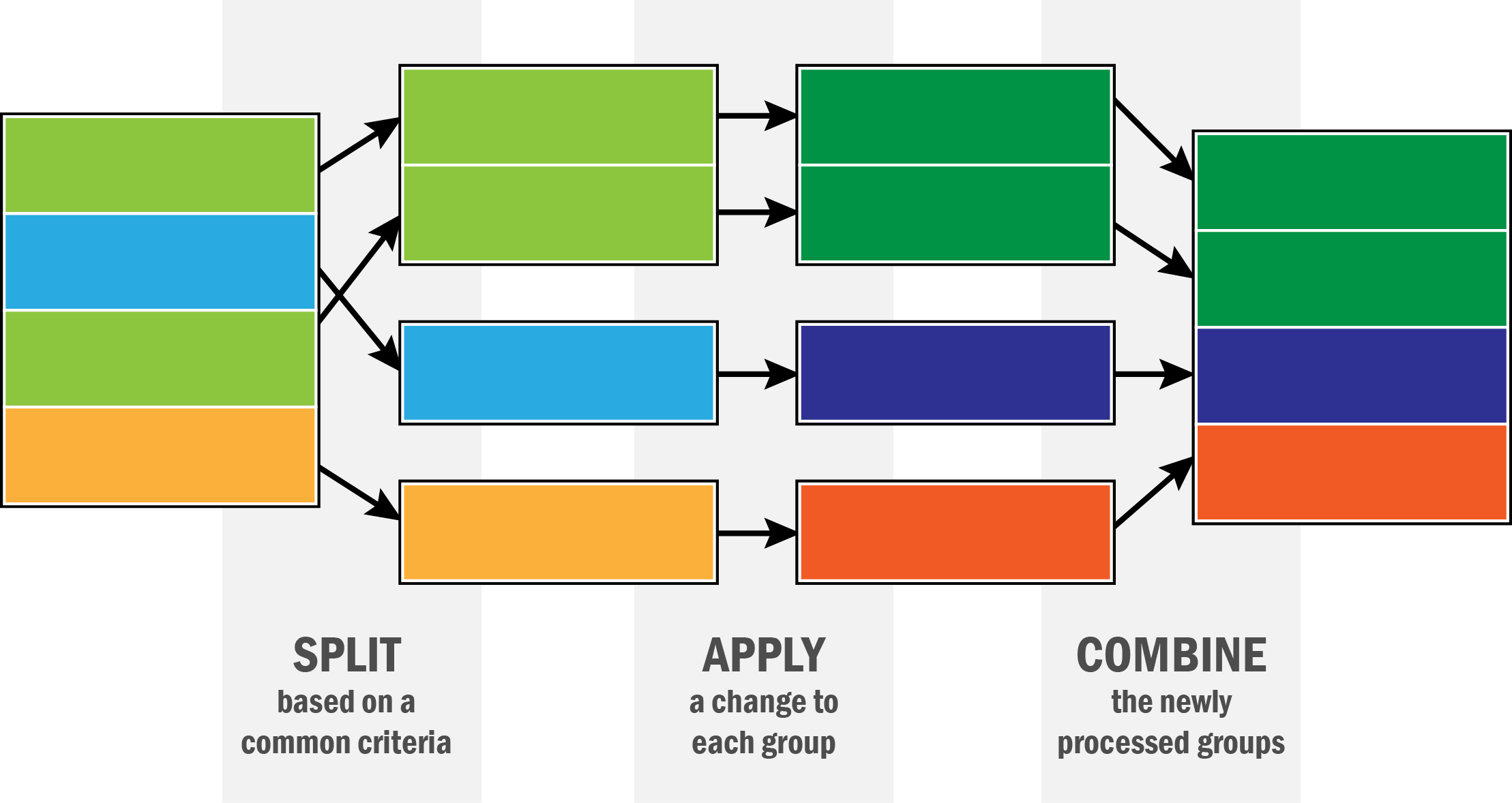
pandas is set up for this. It features the groupby function that allows the “split” part of the operation. We can then apply a function to each part and put it back together. Let’s see how.

df.head()

       country continent  year  lifeExp       pop   gdpPercap
0  Afghanistan      Asia  1952   28.801   8425333  779.445314
1  Afghanistan      Asia  1957   30.332   9240934  820.853030
2  Afghanistan      Asia  1962   31.997  10267083  853.100710
3  Afghanistan      Asia  1967   34.020  11537966  836.197138
4  Afghanistan      Asia  1972   36.088  13079460  739.981106

f"This dataset has {len(df['country'].unique())} countries in it"

'This dataset has 142 countries in it'

One of the variables in this dataset is life expectancy at birth, lifeExp. Suppose we want to find the average life expectancy of each country over the period of study.

df.groupby('country')['lifeExp'].mean()

country
Afghanistan           37.478833
Albania               68.432917
Algeria               59.030167
Angola                37.883500
Argentina             69.060417
                        ...    
Vietnam               57.479500
West Bank and Gaza    60.328667
Yemen, Rep.           46.780417
Zambia                45.996333
Zimbabwe              52.663167
Name: lifeExp, Length: 142, dtype: float64

So what’s going on here? First, we use the groupby function, telling pandas to split the dataset up by values of the column country.

df.groupby('country')

<pandas.core.groupby.generic.DataFrameGroupBy object at 0x11cfb1b50>

pandas won’t show you the actual data, but will tell you that it is a grouped dataframe object. This means that each element of this object is a DataFrame with data from one country.

df.groupby('country').ngroups

df.groupby('country').get_group('United Kingdom')

             country continent  year  lifeExp       pop     gdpPercap
1596  United Kingdom    Europe  1952   69.180  50430000   9979.508487
1597  United Kingdom    Europe  1957   70.420  51430000  11283.177950
1598  United Kingdom    Europe  1962   70.760  53292000  12477.177070
1599  United Kingdom    Europe  1967   71.360  54959000  14142.850890
1600  United Kingdom    Europe  1972   72.010  56079000  15895.116410
1601  United Kingdom    Europe  1977   72.760  56179000  17428.748460
1602  United Kingdom    Europe  1982   74.040  56339704  18232.424520
1603  United Kingdom    Europe  1987   75.007  56981620  21664.787670
1604  United Kingdom    Europe  1992   76.420  57866349  22705.092540
1605  United Kingdom    Europe  1997   77.218  58808266  26074.531360
1606  United Kingdom    Europe  2002   78.471  59912431  29478.999190
1607  United Kingdom    Europe  2007   79.425  60776238  33203.261280

type(df.groupby('country').get_group('United Kingdom'))

<class 'pandas.core.frame.DataFrame'>

avg_lifeexp_country = df.groupby('country').lifeExp.mean()
avg_lifeexp_country['United Kingdom']

73.92258333333332

df.groupby('country').get_group('United Kingdom').lifeExp.mean()

73.92258333333332

Let’s look at if life expectancy has gone up over time, by continent

df.groupby(['continent','year']).lifeExp.mean()

continent  year
Africa     1952    39.135500
           1957    41.266346
           1962    43.319442
           1967    45.334538
           1972    47.450942
           1977    49.580423
           1982    51.592865
           1987    53.344788
           1992    53.629577
           1997    53.598269
           2002    53.325231
           2007    54.806038
Americas   1952    53.279840
           1957    55.960280
           1962    58.398760
           1967    60.410920
           1972    62.394920
           1977    64.391560
           1982    66.228840
           1987    68.090720
           1992    69.568360
           1997    71.150480
           2002    72.422040
           2007    73.608120
Asia       1952    46.314394
           1957    49.318544
           1962    51.563223
           1967    54.663640
           1972    57.319269
           1977    59.610556
           1982    62.617939
           1987    64.851182
           1992    66.537212
           1997    68.020515
           2002    69.233879
           2007    70.728485
Europe     1952    64.408500
           1957    66.703067
           1962    68.539233
           1967    69.737600
           1972    70.775033
           1977    71.937767
           1982    72.806400
           1987    73.642167
           1992    74.440100
           1997    75.505167
           2002    76.700600
           2007    77.648600
Oceania    1952    69.255000
           1957    70.295000
           1962    71.085000
           1967    71.310000
           1972    71.910000
           1977    72.855000
           1982    74.290000
           1987    75.320000
           1992    76.945000
           1997    78.190000
           2002    79.740000
           2007    80.719500
Name: lifeExp, dtype: float64

avg_lifeexp_continent_yr = df.groupby(['continent','year']).lifeExp.mean().reset_index()
avg_lifeexp_continent_yr

   continent  year    lifeExp
0     Africa  1952  39.135500
1     Africa  1957  41.266346
2     Africa  1962  43.319442
3     Africa  1967  45.334538
4     Africa  1972  47.450942
5     Africa  1977  49.580423
6     Africa  1982  51.592865
7     Africa  1987  53.344788
8     Africa  1992  53.629577
9     Africa  1997  53.598269
10    Africa  2002  53.325231
11    Africa  2007  54.806038
12  Americas  1952  53.279840
13  Americas  1957  55.960280
14  Americas  1962  58.398760
15  Americas  1967  60.410920
16  Americas  1972  62.394920
17  Americas  1977  64.391560
18  Americas  1982  66.228840
19  Americas  1987  68.090720
20  Americas  1992  69.568360
21  Americas  1997  71.150480
22  Americas  2002  72.422040
23  Americas  2007  73.608120
24      Asia  1952  46.314394
25      Asia  1957  49.318544
26      Asia  1962  51.563223
27      Asia  1967  54.663640
28      Asia  1972  57.319269
29      Asia  1977  59.610556
30      Asia  1982  62.617939
31      Asia  1987  64.851182
32      Asia  1992  66.537212
33      Asia  1997  68.020515
34      Asia  2002  69.233879
35      Asia  2007  70.728485
36    Europe  1952  64.408500
37    Europe  1957  66.703067
38    Europe  1962  68.539233
39    Europe  1967  69.737600
40    Europe  1972  70.775033
41    Europe  1977  71.937767
42    Europe  1982  72.806400
43    Europe  1987  73.642167
44    Europe  1992  74.440100
45    Europe  1997  75.505167
46    Europe  2002  76.700600
47    Europe  2007  77.648600
48   Oceania  1952  69.255000
49   Oceania  1957  70.295000
50   Oceania  1962  71.085000
51   Oceania  1967  71.310000
52   Oceania  1972  71.910000
53   Oceania  1977  72.855000
54   Oceania  1982  74.290000
55   Oceania  1987  75.320000
56   Oceania  1992  76.945000
57   Oceania  1997  78.190000
58   Oceania  2002  79.740000
59   Oceania  2007  80.719500

type(avg_lifeexp_continent_yr)

<class 'pandas.core.frame.DataFrame'>

The aggregation function, in this case mean, does both the “apply” and “combine” parts of the process.

We can do quick aggregations with pandas

df.groupby('continent').lifeExp.describe()

           count       mean        std  ...      50%       75%     max
continent                               ...                           
Africa     624.0  48.865330   9.150210  ...  47.7920  54.41150  76.442
Americas   300.0  64.658737   9.345088  ...  67.0480  71.69950  80.653
Asia       396.0  60.064903  11.864532  ...  61.7915  69.50525  82.603
Europe     360.0  71.903686   5.433178  ...  72.2410  75.45050  81.757
Oceania     24.0  74.326208   3.795611  ...  73.6650  77.55250  81.235

[5 rows x 8 columns]

df.groupby('continent').nth(10) # Tenth observation in each group

               country  year  lifeExp       pop     gdpPercap
continent                                                    
Africa         Algeria  2002   70.994  31287142   5288.040382
Americas     Argentina  2002   74.340  38331121   8797.640716
Asia       Afghanistan  2002   42.129  25268405    726.734055
Europe         Albania  2002   75.651   3508512   4604.211737
Oceania      Australia  2002   80.370  19546792  30687.754730

You can also use functions from other modules, or your own functions in this aggregation work.

df.groupby('continent').lifeExp.agg(np.mean)

continent
Africa      48.865330
Americas    64.658737
Asia        60.064903
Europe      71.903686
Oceania     74.326208
Name: lifeExp, dtype: float64

def my_mean(values):
    n = len(values)
    sum = 0
    for value in values:
        sum += value
    return(sum/n)

df.groupby('continent').lifeExp.agg(my_mean)

continent
Africa      48.865330
Americas    64.658737
Asia        60.064903
Europe      71.903686
Oceania     74.326208
Name: lifeExp, dtype: float64

You can do many functions at once

df.groupby('year').lifeExp.agg([np.count_nonzero, np.mean, np.std])

      count_nonzero       mean        std
year                                     
1952          142.0  49.057620  12.225956
1957          142.0  51.507401  12.231286
1962          142.0  53.609249  12.097245
1967          142.0  55.678290  11.718858
1972          142.0  57.647386  11.381953
1977          142.0  59.570157  11.227229
1982          142.0  61.533197  10.770618
1987          142.0  63.212613  10.556285
1992          142.0  64.160338  11.227380
1997          142.0  65.014676  11.559439
2002          142.0  65.694923  12.279823
2007          142.0  67.007423  12.073021

You can also aggregate on different columns at the same time by passing a dict to the agg function

df.groupby('year').agg({'lifeExp': np.mean,'pop': np.median,'gdpPercap': np.median}).reset_index()

    year    lifeExp         pop    gdpPercap
0   1952  49.057620   3943953.0  1968.528344
1   1957  51.507401   4282942.0  2173.220291
2   1962  53.609249   4686039.5  2335.439533
3   1967  55.678290   5170175.5  2678.334741
4   1972  57.647386   5877996.5  3339.129407
5   1977  59.570157   6404036.5  3798.609244
6   1982  61.533197   7007320.0  4216.228428
7   1987  63.212613   7774861.5  4280.300366
8   1992  64.160338   8688686.5  4386.085502
9   1997  65.014676   9735063.5  4781.825478
10  2002  65.694923  10372918.5  5319.804524
11  2007  67.007423  10517531.0  6124.371109

4.7.0.1 Transformation

You can do grouped transformations using this same method. We will compute the z-score for each year, i.e. we will substract the average life expectancy and divide by the standard deviation

def my_zscore(values):
    m = np.mean(values)
    s = np.std(values)
    return((values - m)/s)

df.groupby('year').lifeExp.transform(my_zscore)

0      -1.662719
1      -1.737377
2      -1.792867
3      -1.854699
4      -1.900878
          ...   
1699   -0.081910
1700   -0.338167
1701   -1.580537
1702   -2.100756
1703   -1.955077
Name: lifeExp, Length: 1704, dtype: float64

df['lifeExp_z'] = df.groupby('year').lifeExp.transform(my_zscore)

df.groupby('year').lifeExp_z.mean()

year
1952   -5.165078e-16
1957    2.902608e-17
1962    2.404180e-16
1967   -6.108181e-16
1972    1.784566e-16
1977   -9.456442e-16
1982   -1.623310e-16
1987    6.687725e-16
1992    5.457293e-16
1997    8.787963e-16
2002    5.254013e-16
2007    4.925637e-16
Name: lifeExp_z, dtype: float64

4.7.0.2 Filter

We can split the dataset by values of one variable, and filter out those splits that fail some criterion. The following code only keeps countries with a population of at least 10 million at some point during the study period

df.groupby('country').filter(lambda d: d['pop'].max() > 10000000)

          country continent  year  lifeExp       pop   gdpPercap  lifeExp_z
0     Afghanistan      Asia  1952   28.801   8425333  779.445314  -1.662719
1     Afghanistan      Asia  1957   30.332   9240934  820.853030  -1.737377
2     Afghanistan      Asia  1962   31.997  10267083  853.100710  -1.792867
3     Afghanistan      Asia  1967   34.020  11537966  836.197138  -1.854699
4     Afghanistan      Asia  1972   36.088  13079460  739.981106  -1.900878
...           ...       ...   ...      ...       ...         ...        ...
1699     Zimbabwe    Africa  1987   62.351   9216418  706.157306  -0.081910
1700     Zimbabwe    Africa  1992   60.377  10704340  693.420786  -0.338167
1701     Zimbabwe    Africa  1997   46.809  11404948  792.449960  -1.580537
1702     Zimbabwe    Africa  2002   39.989  11926563  672.038623  -2.100756
1703     Zimbabwe    Africa  2007   43.487  12311143  469.709298  -1.955077

[924 rows x 7 columns]