11 Applied machine learning
Last updated: 13 Nov, 2024 08:09 AM EST
Introduction
Machine learning is a catch-all for algorithmic modeling that may incorporate components that account for randomness in the data and measurement errors. Under the umbrella of supervised learning, we find statistical regression modeling, penalized regression models, and other parametric and semi-parametric models in addition to the usual complex “black-box” models usually based on simple learners like decision trees and stubs. The machine learning perspective, though, contrasts with the usual statistical approaches found in biomedical data science in that it emphasizes prediction rather than association. In this chapter, we will consider not only standard classification and regression predictive models, but also models that allow the presence of censored data in the prediction of times till some event, which is a characteristic data type in many biomedical applications.
There is also a well-established spot for unsupervised learning methods in biomedical data science. We saw, when exploring high-dimensional data for biomarker discovery, that cluster analysis is often used to help understand the patterns in the data and often to associate those patterns with other characteristics of subjects. We saw the use of heatmaps and hierarchical clustering in trying to make sense of genomic datasets.
The emphasis in this chapter will be on prediction, following the usual train-test split strategy for model development and validation, and the use of cross-validation for model building. In the next chapter, we will return to the question of associations and causal effects which are often central to the decision-making in biomedical and biological studies.
Supervised learning
We can generally think of supervised machine learning as ways of modeling the regression function \(E(Y|X)\) where \(Y\) is the outcome or response, and \(X\) are the predictors. Additionally, in statistical machine learning, we also specify the random element of the outcome \(Y|X\) via some distribution on the support of \(Y\).
To fix ideas, in classical linear regression, we have \(E(Y|X) = \beta_0 + \beta_1X_1 + \beta_2X_2 + \dots + \beta_pX_p\), with the random element being specified as \(Y|X\sim N(E(Y|X), \sigma^2)\) where \(Y \in \mathbb{R}^n\)
We can model the regression function in a specific function of the predictors (that would include models like linear and logistic regression) or as a flexible functional form of the predictors that embodies a class of models to be learned from the data (including tree-based models, support vector machines), or, in fact, combinations thereof (spline models). We can also combine models into even more flexible and robust models via ensemble methods like bagging, boosting and stacking (superlearners). Each of these are trying to predict \(Y\) from predictors \(X\).
There are two fundamental concepts to help judge models: bias and variance. Bias refers to how “off” our predictions are on average, and variance refers to how much a model would change if we changed some of the data. For example, a linear regression or a decision stub are examples of a high-bias, low-variance model (a straight line can be far off from particular points, but doesn’t change much if we add or subtract some points). On the flip side, a high-degree polynomial model, a deep decision tree are examples of low-bias, high-variance models (they can match the data quite closely, but small changes in the data will change the model significantly). At the extremes, we have a constant function (f(X) = c) and a n-dimensional polynomial for n data points. This exemplifies the so-called bias-variance tradeoff. What we’d like to aim for is a low-bias, low-variance model, which has led to ensemble strategies using high-bias, low-variance base learners; the averaging reduces the bias while keeping the variance low.

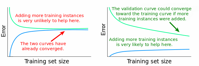
The low-bias aim can lead the models that fit the training data extremely well. In fact, you can think of an interpolating model that fits the data exactly. But that model will fit new data quite poorly; it has overfit the training data. What we want is a model that has learned from the training data well enough, but also provides reasonable predictions on new data. How do we protect against this? We evaluate the performance of models on data the model hasn’t seen before, and see if it still does well. Conceptually, we’ll have to allow slightly higher bias in training the model in order for it to work well on new data. Cross-validation is one approach that allows us to use this process to evaluate models using a single dataset, but we would generally like to validate the model performance on a completely independent data. We can also look at learning curves to see if the training is sufficient or if it would benefit from additional data (if training and test performance are both still increasing).
Predictive models are used in the pharmaceutical industry to help model the risk of individuals to have worse outcomes, or to identify patients more likely to responsd to a treatment regimen. They can be used to help select the “best” patients into a clinical trial to showcase the benefits of a treatment, or inform exclusion criteria to exclude patients from a clinical trial.
So having predictive models which are robust and give good, reliable predictions is important; it can lead to crucial decisions around getting the right patients the right treatments, while not harming patients who would not benefit. So out-of-bag model fit is really considered for these predictive models. These evalutions are also considered by regulatory agencies when the models are used to establish companion diagnostics that are used to determine the safe and effective use of a drug or biologic agent.
These ideas have led to the rise of precision medicine, or the concept of the right treatment for the right patient. It’s certainly not at the level of individualized treatment, but we do today have a better idea of different treatments for different patient segments.
In this chapter we focus mainly on ML for surival analysis, which is unique to BDS. You’ve learned about other machine learning contexts elsewhere in the program.
Caution: use ML models carefully
In this section, I’m primarily referring to ML models of the “black box” ilk, so flexible nonparametric models or ensemble models that are highly complex. These models are known to be data-hungry and require substantial amounts of training data, and correspond amounts of training/validation data, to allow us to develop a properly tuned robust predictive model.
However, in BDS, we often have data sets that are relatively small compared to the massive data sets usually used for ML training. This limited data in a particular experiment or study can lead to overfitting issues and also high predictive variability, neither of which are good things. Moreover, we will often have high-dimensional predictors from genomics or radiomics that make the model fitting even more difficult. So, in the context of BDS, ML models can be quite challenging to develop.
There is a prevailing view that for BDS, we’re better off using smaller statistical parametric models like logistic regression or proportional odds regressions, especially when combined with flexible modeling of the features using spline-based transformations. These models are more defensible and explainable, can be fit adequately with smaller sample sizes due to the restrictions on the functional forms of the models, and can be better predictions with less predictive variability. Yes, this does require competent and skilled model development, but when done well, it can be advantageous.
Frank Harrell, one of my statistical heroes, had written a series of influential blogs and seminars in 2018 on this topic area. Many of the arguments are still valid today in spite of some advances we’ve made in ML.
- Road Map for Choosing Between Statistical Modeling and Machine Learning
- How Can Machine Learning be Reliable When the Sample is Adequate for Only One Feature?
- Is Medicine Mesmerized by Machine Learning?
- Musings on Statistical Models vs. Machine Learning in Health Research
- Controversies in Predictive Modeling, Machine Learning, and Validation
Moving forward with flexible ML models
We’re familiar with the usual models for machine learning that are used for classification and regression tasks. Here we’ll describe models for data typical in BDS, especially in the censored data situation. We’ve already seen parametric and semi-parametric models for censored data, including Cox proportional hazards models and accelerated failure time models. There has been the want to extend these models using more flexible models for the regression model (the “mean” model). The strategy has been to replace the parametric mean model, which is typically linear, with a machine learning model. These have included tree models, random forests, gradient boosting, and more recently, neural networks.
The crucial piece of this enterprise is to define loss functions that will be optimized to fit the ML models to the censored data. Two loss functions are commonly used:
scikit-survival documentation- The Cox partial likelihood loss
This uses the usual loss function in the Cox proportional hazards model, but replaces the linear function \(X\beta\) with a general function \(f(x)\). Let \(T_i\) denote the (potentially censored) event time for subject \(i\), \(\delta_i\) the indicator denoting death or censoring, and \(\mathcal{R}_i\) the risk set at time \(T_i\) (i.e., the individuals still at risk in the population at time \(T_i\)). Then the partial likelihood loss function is defined by
\[ loss = \sum_i \delta_i \left[ f(x_i) - \log\left(\sum_{j\in\mathcal{R}_i}\exp(f(x_j)) \right) \right] \]
and the ML goal is to find a mean function \(\hat{f}\) that minimizes this loss.
- The AFT loss
\[ loss = \sum_{i=1}^n \omega_i (\log y_i - f(x_i)) \] where \(\omega_i = \delta_i/\hat{G}(y_i)\) and \(\hat{G}\) is an estimate of the censoring survival function.
You can also consider two prediction error metrics in addition to the loss functions described above. These metrics are (a) the Harrell concordance (C-) index, and (b) the Brier score. 1
2 Faraggi & Simon (1995), Statistics in Medicine
3 Ishwaran, Kogalur, Blackstone & Lauer (2008), Ann Appl Stat
5 pycox
Several machine learning models have been proposed, mostly using ensemble methods and complex models. Neural networks were proposed as one of the earliest models, but in an era when they were hard to computationally fit2. The censored data extension to random forests was proposed in Breiman’s original paper, but was implemented by Ishwaran, et al3. Gradient boosting has been implemented using the AFT loss function4. There are several implementations of neural networks for survival data5,6
What are we predicting?
First a quick note. You can’t do survival predictions using the usual Cox model. Why?
Now think of any parametric survival model. The regression model predicts parameters in the probability model, which in turn defines the survival function. So, for each individual we can predict values of particular parameters based on the distributional assumptions we’ve made, and those values lead to a particular predicted survival curve.
Continuing on to ML models, we take the same idea. What we’re predicting (or want to predict) are the individual predicted survival curves of individuals. We can then consider the model-averaged survival curve and look at performance features like accuracy and calibration against empirical data.
How are we evaluating models?
The primary metric for evaluating survival models is Harrell’s concordance index or C-index. This measures the proportion of paired observations where the order of the respective survival times is predicted correctly. This measure is agnostic to the scale of the observations since it’s basically a metric based on the ranks of survival times.
The case for statistical learning in this context
Classical ML methods are trained on vast corpuses of data, and result in quite precise predictions. When you don’t have such corpuses, the predictions have a stochastic or random element to them, which we can model. This can be true even for classical ML algorithms. The randomness in the data remains influential in the BDS context and is something ignored by machine learners, who are focused on the prediction problem. Conversely, biostatiticians are quite aware of the variability issues but tend to ignore generalizability of models. BDS requires us to use both our statistical and computer science brains together, bridging Breiman’s “two worlds”.
Harrell’s writings can be the starting point for such an exploration. Thinking through the statistical aspects of ML predictions and the uncertainty of such predictions is quite important as we think about decision-making. Bootstrapping can be one tool to help us understand predictive variability and the potential validity of our predictions.
Bayesian models can also help here. These need to be thought out in the same sense as any parametric model, to be able to reflect our observations. We can do prior and posterior predictive checks to see if our data is well-calibrated. An important aspect of Bayesian models is that they are, by nature, generative. You can simulate new data based on the fitted model quite easily and use that for prediction, and for calibration.
Some modeling points
Adjusting for baseline covariates is a good thing.
Looking at non-linear effects is a good thing. If it doesn’t improve things, you can always go back to the simpler linear model
Encourage estimation rather than testing. Note that ML is basically about estimation and prediction, not about hypothesis testing. Along with uncertainty estimates, this is probably the way to go. Knowledge is on a continuum, and NHST forces it into a dichotomy, which is limiting and incomplete. What is important is that any signal we see sufficiently overcomes the noise so that we can have confidence in our findings.