4 Causal effect estimation
Last updated: 19 Sep, 2024 11:16 AM EDT
Randomized studies
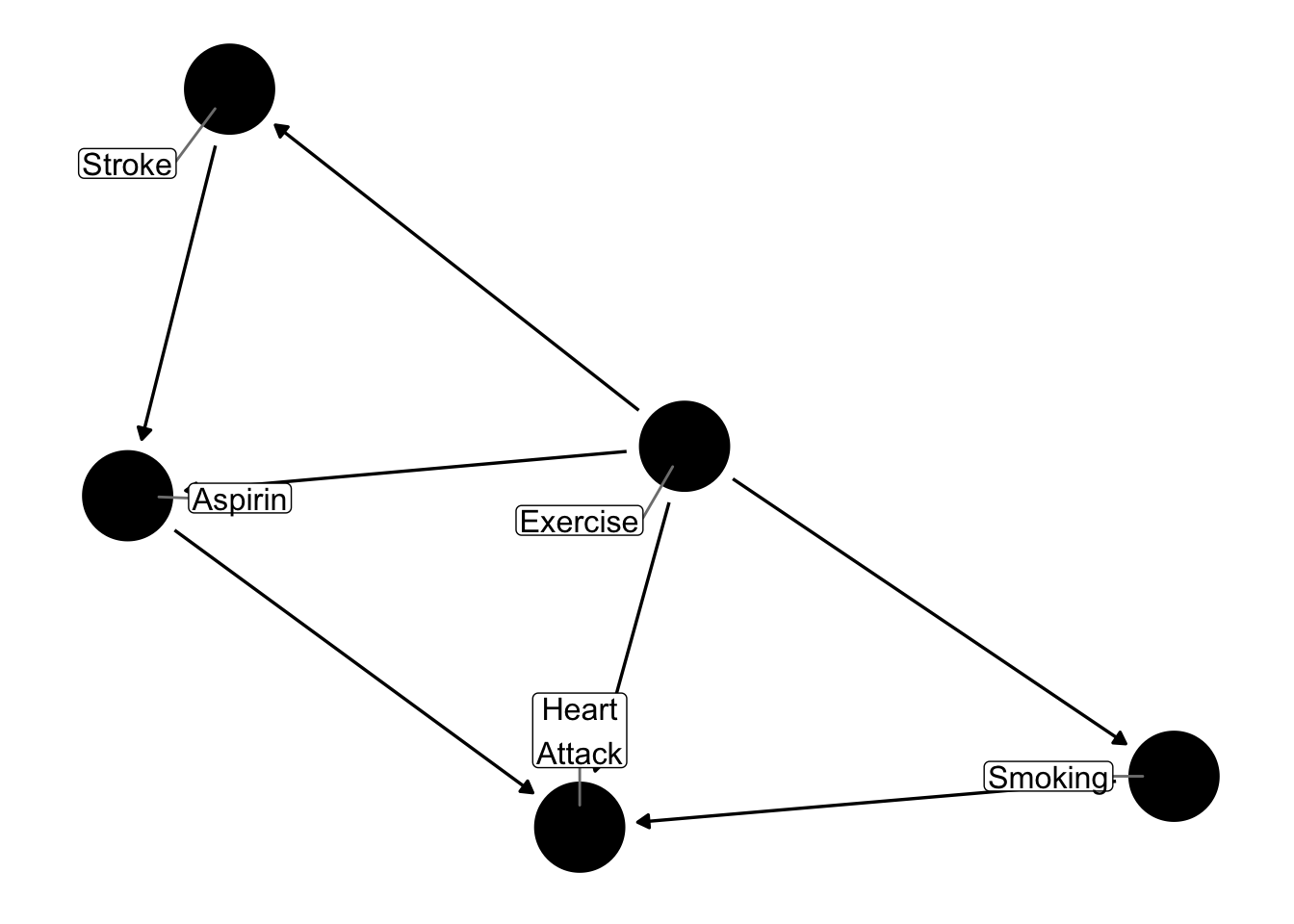
Suppose we have the following causal graph, where we wish to ask the question of whether the use of aspirin affects one’s risk of a heart attack.
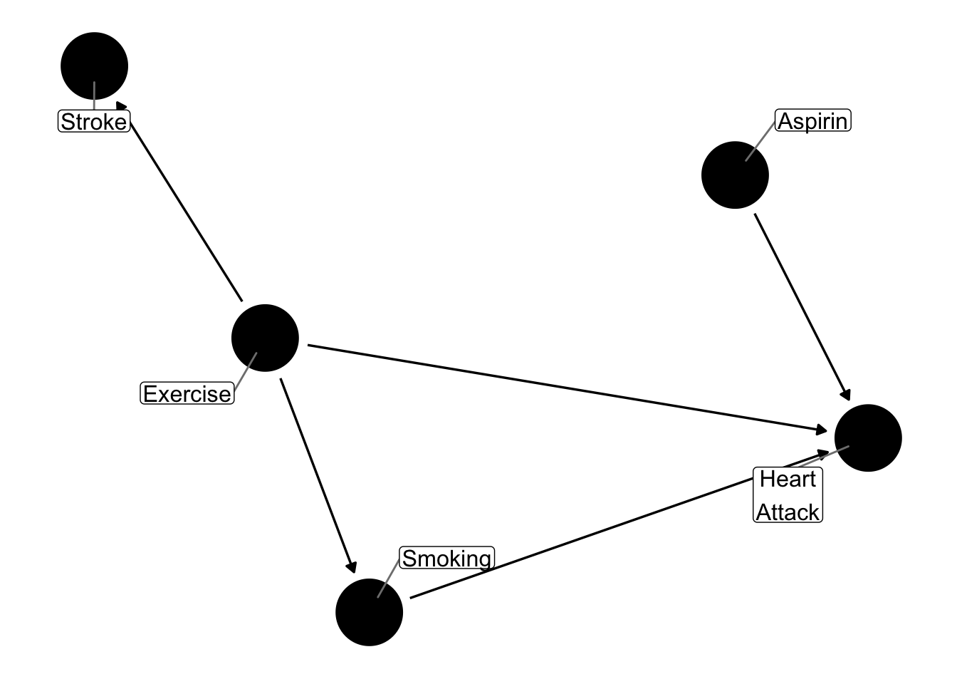
It is clear that there are several backdoor paths between aspirin and heart attack. However, if we randomize the assignment of aspirin in a randomized study, we break all paths to aspirin, and we can consider the following graph, which shows that only the causal path between aspirin and heart attack remains. In the absence of confounders, the observed effect of aspirin on heart attacks in a randomized study is an estimate of the causal effect of aspirin on heart attacks.
The statistical field long held that the only way to assess causal effects was in the randomized study context, which became the gold standard for causal effect assessment. This has, in turn, propagated the use of randomized studies in economics and marketing, where it is often referred to as A/B testing.
However, there are situations when randomized experiments are not feasible or cost prohibitive, or when we have observational data at hand. The question then is, can we analytically estimate causal effects without randomization.
Observational studies
Let’s start by trying to understand what randomized studies achieve. Primarily it is a question of breaking backdoor paths, which is done through balancing potential confounders between those exposed/treated and those not, on average. We can then expect that those confounders no longer act as such since they are no longer empirically associated with the exposure, and the empirical effect of the exposure on the outcome can be interpreted causally.
What if we can achieve similar balance in the confounders in an observational study?
Weighting observations for statistical analysis
We first introduce the concept of weighting. Weighting is commonly used in analyzing survey data to adjust for the way the survey sample is drawn, but the concept is more general. The intent is to create a pseudo-population where the confounders are balanced between levels of the exposure.
Let’s fix ideas with a toy example. In the following figure, we have 3 exposed and 4 non-exposed subjects, and the shading represents the values of a potential confounder.

The central concept we introduce here is that of the propensity score. Propensity refers to the chance of being exposed, given what we know about potential confounders, so, symbolically, \(P(\text{exposed} | \text{confounders})\) . In the above example, we have 1 confounder defined by the shading, and so we have
P(exposed | black) = 1/3
P(exposed | white) = 1/2
The scheme we now introduce is called Inverse Probability of Treatment Weights (IPTW). We will weight each exposed unit by the inverse of the probability of being exposed given the confounder’s value, and similarly we will weight each non-exposed unit by the inverse of the probability of being not exposed. This results in the following weights:
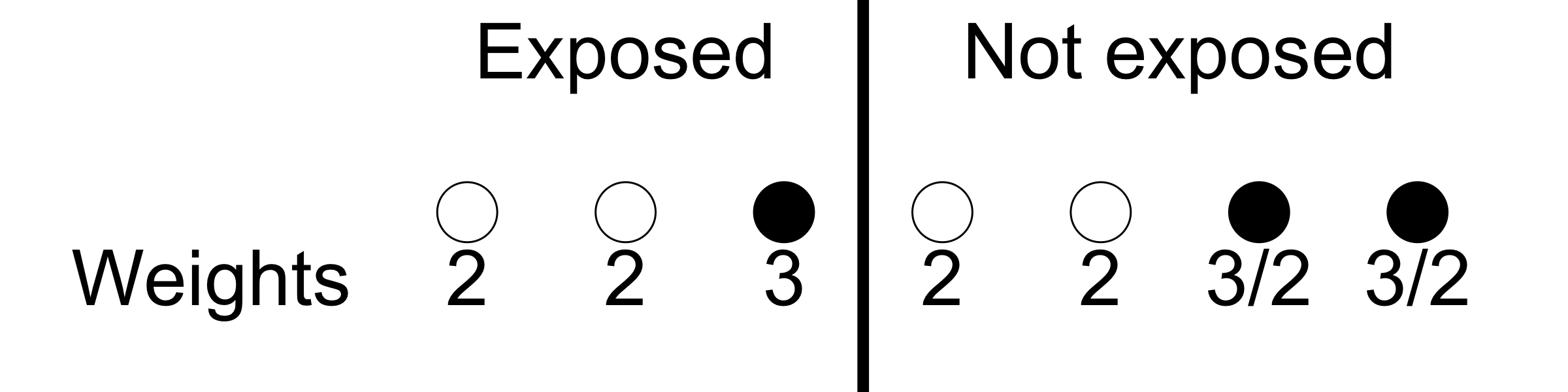
The effect of the weights is effectively to clone the units, even fractionally. This gets us to the following pseudo-population where the confounders are balanced and so their effect in biasing the causal effect of interest is removed.

Propensity scores
The propensity score is defined as P(exposed | confounders). In the previous section, we see how this works for a single binary confounder. Now we need to extend this concept to the situation where we have multiple confounders, possibly of different data types. The core idea is that we find an estimate of P(exposure | confounders) for all possible value combinations of confounder values, and then use the IPTW scheme to weight the units based on these scores.
We can address this problem using regression models or supervised learning models. For binary outcomes, we typically use logistic regression, but other supervised learning choices like random forests, GBM, nearest neighbors, are also usable. We note here that we are developing a model to estimate the probability of being exposed based on potential confounders; this model does not include the outcome at all.
Regression models are basically meant to model E(Y|X), which is also called the regression function as a function of (potentially multivariate) X. In linear models we impose a particular functional form to estimate E(Y|X), but black box supervised learning models attempt to do the same thing.
We note here that P(Y|X) = E(Y|X) when Y is binary (i.e. takes values 0 and 1), and so estimating P(Y|X) can be seen as a regression problem as well.