class: center, middle, inverse, title-slide # Putting it together ### Abhijit Dasgupta, PhD --- layout: true <div class="my-header"> <span style="left: 15px; bottom:2px;">BIOF 439: Data Visualization with R</span> <span style='right:15px; bottom:2px;'>Abhijit Dasgupta</span> </div> --- class: middle, center # Customization --- ## Colors ggplot2 has several ways to customize colors 1. If colors are based on categorical data - `scale_color_manual` - `scale_fill_manual` 1. If colors are based on continuous data - `scale_{color,fill}_gradient` makes sequential gradients (specify low and high colors) - `scale_{color,fill}_gradient2` makes divergent gradients (specify low, middle and high colors) --- ## Colors .pull-left[ ```r (g1 <- ggplot(diamonds, aes(x = cut, y = price, color = carat))+ geom_jitter() ) ``` ] .pull-right[ 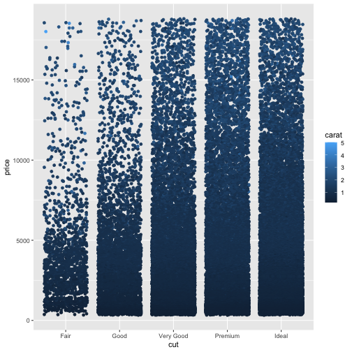<!-- --> ] --- ## Colors .pull-left[ ```r g1 + scale_color_gradient(low='white',high = 'red') ``` ] .pull-right[ 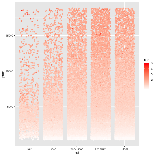<!-- --> ] --- ## Colors .pull-left[ ```r g1 + scale_color_gradient2(low = 'blue', mid='white', high='red', midpoint = 2) ``` ] .pull-right[ 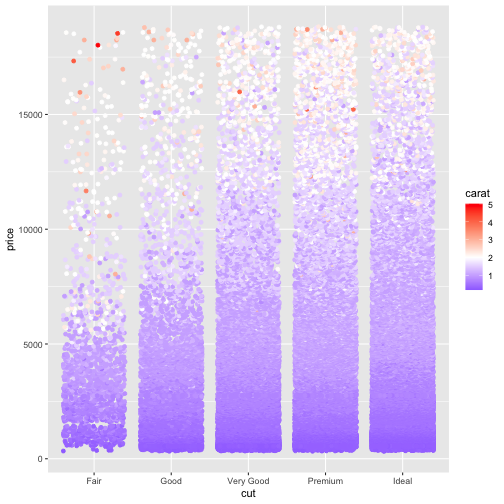<!-- --> ] --- ## Text The `extrafont` package allows you to use fonts already on your computer in your graphics. .pull-left[ ```r library(extrafont) loadfonts() g1 + theme(text = element_text(family='Georgia')) ``` ] .pull-right[ 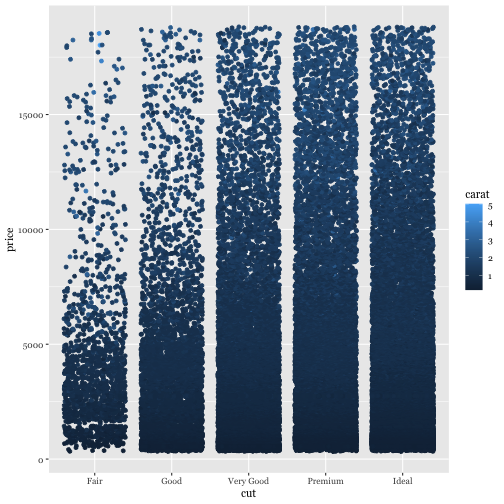<!-- --> ] --- ## Text The `extrafont` package allows you to use fonts already on your computer in your graphics. .pull-left[ ```r g1 + theme(text = element_text(family='Comic Sans MS', size=14)) ``` ] .pull-right[ <!-- --> ] --- class: middle, center # Saving your work --- ## File types .pull-left[ ### Raster - PNG, TIFF, JPEG - Have to specify a resolution (dots per inch or dpi) - Enlarging a file can create pixelation - Preferred for web ] .pull-right[ ### Vector - PDF, SVG, EMF - Infinite resolution - No pixelation - Preferred for print ] --- ## Saving your work Generally, in `ggplot2`, you can use the `ggsave` function with a file name. It figures out the file type from the last letters ```r ggsave('test1.pdf', plot = g1) ggsave('test1.tiff', plot = g1) ``` If you're saving the last graph rendered, you don't need the `plot = g1` part. You can also specify height and width of the graph. --- ## A note about TIFF files TIFF files are not saved with the proper resolution from R. It defaults to 72 dpi, which is inadequate for publication. Save your graph as PDF, and then use Acrobat or Illustrator to change it to a TIFF file with appropriate resolution. Also, make sure that you use __LZW__ compression, otherwise the TIFF file will be unreasonably large. > I have some scripts that I can make available for conversion --- class: middle, center # Creating a final product --- ## R Markdown [R Markdown](https://rmarkdown.rstudio.com) is a lightweight markup language that can inter-weave text and R code to create different kinds of outputs. The [formats page](https://rmarkdown.rstudio.com/formats.html) gives you the breadth of documents that can be generated using R Markdown. --- ## R Markdown You can directly create PowerPoint presentations from R Markdown. This may be useful for your final presentations To create PDF documents, you must have LaTeX installed. This can be achieved by installing the `tinytex` package in R. Or, you can install [MikTeX](https://miktex.org) on Windows or [MacTeX](http://www.tug.org/mactex) on Mac OS X. --- class: middle, center, inverse # Demos --- ## Dashboard The `flexdashboard` package can help create interactive dashboards using R Markdown. The example we will use is based on [this](https://github.com/DIYtranscriptomics/DIYtranscriptomics.github.io/blob/master/Code/files/flexdashboard_essentials.Rmd) flexdashboard example. The data I use is also in that repository.