class: center, middle, inverse, title-slide # Data validation and exploration ### Abhijit Dasgupta ### BIOF 339 --- layout: true <div class="my-header"> <span>BIOF 339: Practical R</span> </div> --- ## Plan today - Dynamic exploration of data - Data validation - Missing data evaluation --- class: middle, center # Why go back to this? --- ## This is important!! + Most of the time in an analysis is spent understanding and cleaning data + Recognize that unless you've ended up with good-quality data, the rest of the analyses are moot + This is tedious, careful, non-sexy work - Hard to tell your boss you're still fixing the data - No real results yet - But essential to understanding the appropriate analyses and the tweaks you may need. --- ## What does a dataset look like? .pull-left[ ```r library(tidyverse) library(visdat) beaches <- rio::import('../data/sydneybeaches3.csv') vis_dat(beaches) ``` ] .pull-right[ <!-- --> ] --- ## What does a dataset look like? .pull-left[ ```r brca <- rio::import('../data/clinical_data_breast_cancer_modified.csv') vis_dat(brca) ``` ] .pull-right[ <!-- --> ] --- ## What does a dataset look like? .pull-left[ ```r vis_dat(airquality) ``` These plots give a nice insight into 1. data types 1. Missing data patterns (more on this later) ] .pull-right[ <!-- --> ] --- class: middle, center # Let's get a bit more quantitative --- ## `summary` and `str`/`glimpse` are a first pass .pull-left[ ```r summary(airquality) ``` ``` Ozone Solar.R Wind Temp Min. : 1.00 Min. : 7.0 Min. : 1.700 Min. :56.00 1st Qu.: 18.00 1st Qu.:115.8 1st Qu.: 7.400 1st Qu.:72.00 Median : 31.50 Median :205.0 Median : 9.700 Median :79.00 Mean : 42.13 Mean :185.9 Mean : 9.958 Mean :77.88 3rd Qu.: 63.25 3rd Qu.:258.8 3rd Qu.:11.500 3rd Qu.:85.00 Max. :168.00 Max. :334.0 Max. :20.700 Max. :97.00 NA's :37 NA's :7 Month Day Min. :5.000 Min. : 1.0 1st Qu.:6.000 1st Qu.: 8.0 Median :7.000 Median :16.0 Mean :6.993 Mean :15.8 3rd Qu.:8.000 3rd Qu.:23.0 Max. :9.000 Max. :31.0 ``` ] .pull-right[ ```r glimpse(airquality) ``` ``` Rows: 153 Columns: 6 $ Ozone <int> 41, 36, 12, 18, NA, 28, 23, 19, 8, NA, 7, 16, 11, 14, 18, 14, … $ Solar.R <int> 190, 118, 149, 313, NA, NA, 299, 99, 19, 194, NA, 256, 290, 27… $ Wind <dbl> 7.4, 8.0, 12.6, 11.5, 14.3, 14.9, 8.6, 13.8, 20.1, 8.6, 6.9, 9… $ Temp <int> 67, 72, 74, 62, 56, 66, 65, 59, 61, 69, 74, 69, 66, 68, 58, 64… $ Month <int> 5, 5, 5, 5, 5, 5, 5, 5, 5, 5, 5, 5, 5, 5, 5, 5, 5, 5, 5, 5, 5,… $ Day <int> 1, 2, 3, 4, 5, 6, 7, 8, 9, 10, 11, 12, 13, 14, 15, 16, 17, 18,… ``` ] --- ## Validating data values + We can certainly be reactive by just describing the data and looking for anomalies. + For larger data or multiple data files it makes sense to be proactive and catch errors that you want to avoid, before exploring for new errors. + The `assertthat` package provides nice tools to do this -- > **Note to self:** I don't do this enough. This is a good defensive programming technique that can catch crucial problems that aren't always automatically flagged as errors --- ## Being assertive ```r library(assertthat) assert_that(all(between(airquality$Day, 1, 31) )) ``` ``` [1] TRUE ``` ```r assert_that(is.factor(mpg$manufacturer)) ``` ``` Error: mpg$manufacturer is not a factor ``` ```r assert_that(all(beaches$season_name %in% c('Summer','Winter','Spring', 'Fall'))) ``` ``` Error: Elements 11, 12, 13, 14, 15, ... of beaches$season_name %in% c("Summer", "Winter", "Spring", "Fall") are not true ``` --- ## Being assertive + `assert_that` generates an error, which will stop things + `see_if` does the same validation, but just generates a `TRUE/FALSE`, which you can capture ```r see_if(is.factor(mpg$manufacturer)) ``` ``` [1] FALSE attr(,"msg") [1] "mpg$manufacturer is not a factor" ``` + `validate_that` generates `TRUE` if the assertion is true, otherwise generates a string explaining the error ```r validate_that(is.factor(mpg$manufacturer)) ``` ``` [1] "mpg$manufacturer is not a factor" ``` ```r validate_that(is.character(mpg$manufacturer)) ``` ``` [1] TRUE ``` --- ## Being assertive You can even write your own validation functions and custom messages ```r is_odd <- function(x){ assert_that(is.numeric(x), length(x)==1) x %% 2 == 1 } assert_that(is_odd(2)) ``` ``` Error: is_odd(x = 2) is not TRUE ``` ```r on_failure(is_odd) <- function(call, env) { paste0(deparse(call$x), " is even") # This is a R trick } assert_that(is_odd(2)) ``` ``` Error: 2 is even ``` ```r is_odd(1:2) ``` ``` Error: length(x) not equal to 1 ``` --- class: middle,center # Missing data --- ## Missing data R denotes missing data as `NA`, and supplies several functions to deal with missing data. The most fundamental is `is.na`, which gives a TRUE/FALSE answer ```r is.na(NA) ``` ``` [1] TRUE ``` ```r is.na(25) ``` ``` [1] FALSE ``` --- ## Missing data When we get a new dataset, it's useful to get a sense of the missingness ```r mpg %>% summarize(across(everything(), function(x) sum(is.na(x)))) ``` ``` # A tibble: 1 × 11 manufacturer model displ year cyl trans drv cty hwy fl class <int> <int> <int> <int> <int> <int> <int> <int> <int> <int> <int> 1 0 0 0 0 0 0 0 0 0 0 0 ``` --- ## Missing data The `naniar` package allows a tidyverse-compatible way to deal with missing data ```r library(naniar) weather <- rio::import('../data/weather.csv') all_complete(mpg) ``` ``` [1] TRUE ``` ```r all_complete(weather) ``` ``` [1] FALSE ``` ```r weather %>% summarize_all(pct_complete) ``` ``` id year month element d1 d2 d3 d4 d5 d6 1 100 100 100 100 9.090909 18.18182 18.18182 9.090909 36.36364 9.090909 d7 d8 d9 d10 d11 d12 d13 d14 d15 1 9.090909 9.090909 0 9.090909 9.090909 0 9.090909 18.18182 9.090909 d16 d17 d18 d19 d20 d21 d22 d23 d24 d25 d26 d27 1 9.090909 9.090909 0 0 0 0 0 18.18182 0 9.090909 9.090909 27.27273 d28 d29 d30 d31 1 9.090909 18.18182 9.090909 9.090909 ``` --- ## Missing data ```r gg_miss_case(weather, show_pct = T) ``` <!-- --> --- ## Missing data ```r gg_miss_var(weather, show_pct=T) ``` ``` Warning: It is deprecated to specify `guide = FALSE` to remove a guide. Please use `guide = "none"` instead. ``` 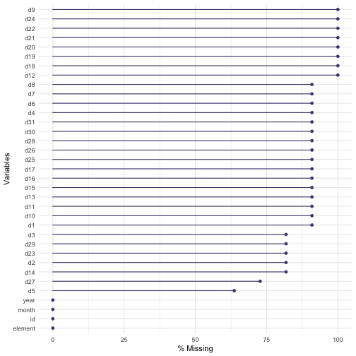<!-- --> --- ## Are there patterns to the missing data + Most analyses assume that data is either - Missing completely at random (MCAR) - Missing at random (MAR) + MCAR means - The missing data is just a random subset of the data + MAR means - Whether data is missing is related to values of some other variable(s) - If we control for those variable(s), the missing data would form a random subset of each of those data subsets defined by unique values of these variables --- ## Are there patterns to the missing data #### MAR or MCAR allows us to ignore the missing data, since it doesn't bias our analyses #### If data are **not** MCAR or MAR, we really need to understand the issing data mechanism and how that might affect our results. --- ## Co-patterns of missingness .pull-left[ ```r gg_miss_upset(airquality) ``` 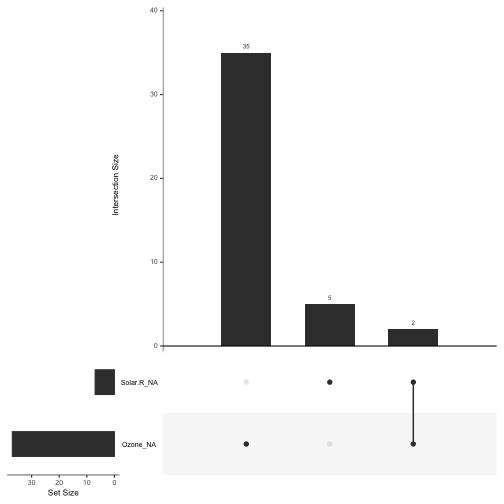<!-- --> ] .pull-right[ ```r gg_miss_upset(riskfactors) ``` 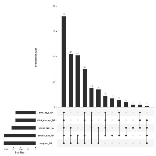<!-- --> ] --- ## Co-patterns of missingness .pull-left[ ```r ggplot(airquality, aes(x = Ozone, y = Solar.R)) + geom_point() ``` ``` Warning: Removed 42 rows containing missing values (geom_point). ``` 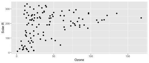<!-- --> ] .pull-right[ ```r ggplot(airquality, aes(x = Ozone, y = Solar.R)) + geom_miss_point() ``` <!-- --> ] --- ## Co-patterns of missingness ```r gg_miss_fct(x = riskfactors, fct = marital) ``` <!-- --> --- ## Replacing missing data `tidyr` has a function `replace_na` which will replace all missing values with some particular value. In the weather dataset, values are missing generally because there wasn't recorded rainfall on a day. So these values should really be 0 ```r weather1 <- weather %>% mutate(d1 = replace_na(d1, 0)) pct_miss(weather1$d1) ``` ``` [1] 0 ``` --- ### Question: How would you replace all the missing values with 0? -- ```r weather %>% mutate(across(everything(),function(x) replace_na(x, 0))) ``` -- ### How would you replace the missing values with the mean of the variable? -- ```r weather %>% mutate(across(where(is.numeric), function(x) replace_na(x, mean(x, na.rm=T)))) ``` ---