Joins, summaries and subgroups

class: center, middle, inverse, title-slide

# Joins, summaries and subgroups
### Abhijit Dasgupta
### March 25-27, 2019

---

layout: true

<div class="my-header">
<span>PS 312, March 2019</span></div>

---
class: middle, center, inverse

# Welcome to Day 2

---

# More about `select`

`select` selects variables from your dataset.

__Usage__: dataset %>% select(variable names)

```r
library(rio)
dos <- import('Data/FSI/Department of State.csv') %>% as_tibble()
# names(dos)
```

This data set has variables in various groups by name.

---

# More about `select`

.left-column30[

```r
dos %>% 
  select(starts_with("Award"))
```
]
.right-column30[

```
# A tibble: 558,878 x 24
   Award_Identifier Award_Title Award_Descripti… Award_Status
   <chr>            <chr>       <chr>            <chr>       
 1 1040240201       ""          Ambassadors-At-… Implementat…
 2 1040240201       ""          Ambassadors-At-… Implementat…
 3 1040240201       ""          Ambassadors-At-… Implementat…
 4 1040240220       ""          Ambassadors-At-… Implementat…
 5 1040240202       ""          Ambassadors-At-… Implementat…
 6 1040240202       ""          Ambassadors-At-… Implementat…
 7 1040240204       ""          Ambassadors-At-… Implementat…
 8 1040240204       ""          Ambassadors-At-… Implementat…
 9 1040240225       ""          Ambassadors-At-… Implementat…
10 1040240225       ""          Ambassadors-At-… Implementat…
# … with 558,868 more rows, and 20 more variables:
#   Award_Collaboration_Type <chr>, Award_Total_Estimated_Value <dbl>,
#   Award_Interagency_Transfer_Status <chr>, Award_Start_Date <chr>,
#   Award_End_Date <chr>, Award_Transaction_Description <chr>,
#   Award_Transaction_Value <dbl>, Award_Transaction_Type <chr>,
#   Award_Transaction_Date <chr>, Award_Transaction_Fiscal_Year <int>,
#   Award_Transaction_Fiscal_Quarter <int>,
#   Award_Transaction_Aid_Type <chr>, Award_Transaction_Tied_Status <chr>,
#   Award_Transaction_Flow_Type <chr>,
#   Award_Transaction_Finance_Type <chr>,
#   Award_Transaction_DAC_Purpose_Code <int>,
#   Award_Transaction_DAC_Purpose_Code_Name <chr>,
#   Award_Transaction_US_Foreign_Assistance_Code <int>,
#   Award_Transaction_US_Foreign_Assistance_Category <chr>,
#   Award_Transaction_US_Foreign_Assistance_Sector <chr>
```

]
---

# More about `select`

.left-column30[

```r
dos %>% 
  select(ends_with("Value"))
```
]
.right-column30[

```
# A tibble: 558,878 x 2
   Award_Total_Estimated_Value Award_Transaction_Value
                         <dbl>                   <dbl>
 1                           0                    194.
 2                           0                    301.
 3                           0                    287.
 4                           0                   2470.
 5                           0                   1031.
 6                           0                   2853.
 7                           0                   3431.
 8                           0                    912.
 9                           0                    525.
10                           0                   1436.
# … with 558,868 more rows
```

]
---

# More about `select`

.left-column30[

```r
dos %>% 
  select(contains("Transaction"))
```
]
.right-column30[

```
# A tibble: 558,878 x 15
   Award_Transacti… Award_Transacti… Award_Transacti… Award_Transacti…
   <chr>                       <dbl> <chr>            <chr>           
 1 ""                           194. Disbursement     2011-11-30 00:0…
 2 ""                           301. Commitment       2011-10-31 00:0…
 3 ""                           287. Disbursement     2011-10-31 00:0…
 4 ""                          2470. Commitment       2011-10-31 00:0…
 5 ""                          1031. Commitment       2011-11-30 00:0…
 6 ""                          2853. Disbursement     2011-11-30 00:0…
 7 ""                          3431. Disbursement     2011-12-31 00:0…
 8 ""                           912. Disbursement     2011-11-30 00:0…
 9 ""                           525. Commitment       2011-12-31 00:0…
10 ""                          1436. Disbursement     2011-12-31 00:0…
# … with 558,868 more rows, and 11 more variables:
#   Award_Transaction_Fiscal_Year <int>,
#   Award_Transaction_Fiscal_Quarter <int>,
#   Award_Transaction_Aid_Type <chr>, Award_Transaction_Tied_Status <chr>,
#   Award_Transaction_Flow_Type <chr>,
#   Award_Transaction_Finance_Type <chr>,
#   Award_Transaction_DAC_Purpose_Code <int>,
#   Award_Transaction_DAC_Purpose_Code_Name <chr>,
#   Award_Transaction_US_Foreign_Assistance_Code <int>,
#   Award_Transaction_US_Foreign_Assistance_Category <chr>,
#   Award_Transaction_US_Foreign_Assistance_Sector <chr>
```

]

---

# `select` helpers

- starts_with(): Starts with a prefix.
- ends_with(): Ends with a suffix.
- contains(): Contains a literal string.
- matches(): Matches a regular expression.
- num_range(): Matches a numerical range like x01, x02, x03.
- one_of(): Matches variable names in a character vector.
- everything(): Matches all variables.
- last_col(): Select last variable, possibly with an offset.

---

# Dates

```r
start_dates <-  dos %>% 
  select(ends_with("Date")) %>% 
  select(contains("Start")) %>% 
  pull(1)
  
head(start_dates)
```

```
[1] "2011-10-05 00:00:00" "2011-10-05 00:00:00" "2011-10-05 00:00:00"
[4] "2011-10-21 00:00:00" "2011-10-03 00:00:00" "2011-10-03 00:00:00"
```

Let's work a bit with dates

Cheatsheet: [https://rawgit.com/rstudio/cheatsheets/master/lubridate.pdf](https://rawgit.com/rstudio/cheatsheets/master/lubridate.pdf)

---

# Dates

```r
library(lubridate)
start_dates <- as_date(start_dates) %>% head()
start_dates
```

```
[1] "2011-10-05" "2011-10-05" "2011-10-05" "2011-10-21" "2011-10-03"
[6] "2011-10-03"
```

```r
year(start_dates)
```

```
[1] 2011 2011 2011 2011 2011 2011
```

```r
month(start_dates)
```

```
[1] 10 10 10 10 10 10
```

```r
day(start_dates)
```

```
[1]  5  5  5 21  3  3
```

---

# Dates

```r
sort(start_dates)
```

```
[1] "2011-10-03" "2011-10-03" "2011-10-05" "2011-10-05" "2011-10-05"
[6] "2011-10-21"
```

```r
quarter(start_dates)
```

```
[1] 4 4 4 4 4 4
```

```r
days(start_dates) - days(as_date('2011-10-01')) # Days from start of fiscal year
```

```
[1] "4d 0H 0M 0S"  "4d 0H 0M 0S"  "4d 0H 0M 0S"  "20d 0H 0M 0S"
[5] "2d 0H 0M 0S"  "2d 0H 0M 0S" 
```

---
class: middle, center

# Joins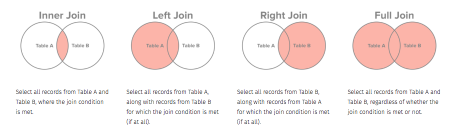

---

![](img/joins.png)

---

# Some simulated data

We simulated 2 datasets
- real estate allocation at DOS by Bureau
- staffing at DOS by Bureau

We want to see what the average area per person is across DOS

```r
staffing_data <- import('Data/FSI/Staffing_by_Bureau.csv')
real_estate <- import('Data/FSI/DoS_Real_Estate_Allocation.csv')
```

---

```r
staffing_data %>% as_tibble()
```

```
# A tibble: 10,000 x 6
   Bureau                      Gender Grade Title    Name      YearsService
   <chr>                       <chr>  <chr> <chr>    <chr>            <int>
 1 Protocol (S/CPR)            female FS1   Manager  Cathy Ca…           13
 2 Administration (A)          male   GS-9  Team Me… Jeffery …           13
 3 Intelligence and Research … male   FS-6  Analyst  Max Green           11
 4 Mission to the United Nati… male   FS-3  Manager  Donald A…            7
 5 Foreign Missions (OFM)      male   FS-6  Team Me… Thomas L…           22
 6 International Narcotics an… male   GS-8  Team Me… Joseph A…           12
 7 Administration (A)          male   GS-12 Analyst  Michael …            6
 8 Intelligence and Research … male   FS-5  Team Me… Jesus Sh…            2
 9 Science & Technology Advis… male   N/A   Manager  Lawrence…           19
10 Administration (A)          female FS-8  Team Me… Jennie C…           17
# … with 9,990 more rows
```

```r
real_estate %>% as_tibble()
```

```
# A tibble: 666 x 4
   Building Bureau               Location  Size
   <chr>    <chr>                   <int> <int>
 1 HST      Administration (A)       4779   640
 2 SA2      Administration (A)       4801  1090
 3 HST      Administration (A)       5109  1040
 4 HST      Administration (A)       3717  1620
 5 SA4      Administration (A)       3940  1390
 6 HST      Administration (A)       3661  1480
 7 HST      Administration (A)       3374  1770
 8 HST      Administration (A)       3387  1940
 9 SA10     African Affairs (AF)     2605   640
10 HST      African Affairs (AF)     3573   720
# … with 656 more rows
```

---

```r
staff_summary <- staffing_data %>% 
  group_by(Bureau) %>% 
  tally(name = 'Pop')
realestate_summary <- real_estate %>% 
 group_by(Bureau) %>% summarize(Size = sum(Size))
```

```r
staff_summary %>% head(4)
```

```
# A tibble: 4 x 2
  Bureau                                            Pop
  <chr>                                           <int>
1 Administration (A)                                454
2 African Affairs (AF)                               42
3 Allowances (A/OPR/ALS)                             90
4 Arms Control, Verification and Compliance (AVC)    98
```

```r
realestate_summary %>% head(4)
```

```
# A tibble: 4 x 2
  Bureau                                           Size
  <chr>                                           <int>
1 Administration (A)                              10970
2 African Affairs (AF)                            26750
3 Allowances (A/OPR/ALS)                           3010
4 Arms Control, Verification and Compliance (AVC)  8410
```

---

```r
staff_summary %>% 
  inner_join(realestate_summary, by = c("Bureau" = "Bureau"))
```

```
# A tibble: 54 x 3
   Bureau                                             Pop  Size
   <chr>                                            <int> <int>
 1 Administration (A)                                 454 10970
 2 African Affairs (AF)                                42 26750
 3 Allowances (A/OPR/ALS)                              90  3010
 4 Arms Control, Verification and Compliance (AVC)     98  8410
 5 Budget and Planning (BP)                           168  7500
 6 Chief Information Officer (CIO)                    222 11390
 7 Comptroller and Global Financial Services (CGFS)   169 15700
 8 Conflict and Stabilization Operations (CSO)        392 14970
 9 Consular Affairs (CA)                              141 36610
10 Counterterrorism (CT)                              324  9980
# … with 44 more rows
```

---

```r
staff_summary %>% 
  inner_join(realestate_summary, by = c("Bureau" = "Bureau")) %>% 
  mutate(unit_area = Size/Pop) %>% 
  arrange(unit_area)
```

```
# A tibble: 54 x 4
   Bureau                                               Pop  Size unit_area
   <chr>                                              <int> <int>     <dbl>
 1 Global Youth Issues (GYI)                            345  2090      6.06
 2 Policy Planning Staff (S/P)                          240  2420     10.1 
 3 Science & Technology Adviser (STAS)                  305  4240     13.9 
 4 Foreign Missions (OFM)                               311  4420     14.2 
 5 Trafficking in Persons (TIP)                         247  5150     20.9 
 6 Medical Services (MED)                               308  6760     21.9 
 7 Protocol (S/CPR)                                     327  7730     23.6 
 8 Administration (A)                                   454 10970     24.2 
 9 Oceans and International Environmental and Scient…   330  8420     25.5 
10 Energy Resources (ENR)                               369 10890     29.5 
# … with 44 more rows
```

---
class: middle, center

# Summarizing data

---

# The `dplyr` package

This gives us 5 verbs for single data frames:

- `filter`: filter a dataset by rows
- `select`: select columns of a dataset
- `arrange`: arrange rows of a dataset by values of some variables
- `group_by`: split a dataset by values of some variables, so that we can apply verbs to each split
- `summarize`: compute various summaries from the data

---

# The `dplyr` package

.pull-left[
Gives us verbs for joining 2 data frames:

- `left_join`
- `right_join`
- `inner_join`
- `outer_join`
- `semi_join`
- `anti_join`
- `bind_rows`
- `bind_cols`
]
.pull-right[
The joins are different ways to merge two data sets which have at least one variable in common

The `semi-join` and `anti-join` are really filters rather than joins

The last two just put data frames together as long as they conform in dimension
]

---

```r
library(tidyverse)
mtcars1 <- mtcars %>% rownames_to_column('cars') %>% as_tibble()
mtcars1
```

```
# A tibble: 32 x 12
   cars    mpg   cyl  disp    hp  drat    wt  qsec    vs    am  gear  carb
   <chr> <dbl> <dbl> <dbl> <dbl> <dbl> <dbl> <dbl> <dbl> <dbl> <dbl> <dbl>
 1 1      21       6  160    110  3.9   2.62  16.5     0     1     4     4
 2 2      21       6  160    110  3.9   2.88  17.0     0     1     4     4
 3 3      22.8     4  108     93  3.85  2.32  18.6     1     1     4     1
 4 4      21.4     6  258    110  3.08  3.22  19.4     1     0     3     1
 5 5      18.7     8  360    175  3.15  3.44  17.0     0     0     3     2
 6 6      18.1     6  225    105  2.76  3.46  20.2     1     0     3     1
 7 7      14.3     8  360    245  3.21  3.57  15.8     0     0     3     4
 8 8      24.4     4  147.    62  3.69  3.19  20       1     0     4     2
 9 9      22.8     4  141.    95  3.92  3.15  22.9     1     0     4     2
10 10     19.2     6  168.   123  3.92  3.44  18.3     1     0     4     4
# … with 22 more rows
```
--

```r
mtcars1 %>% summarize(mpg = mean(mpg, na.rm=T), disp = mean(disp, na.rm=T), hp = mean(hp, na.rm=T))
```

```
# A tibble: 1 x 3
    mpg  disp    hp
  <dbl> <dbl> <dbl>
1  20.1  231.  147.
```

---

# Scoped verbs

All the `dplyr` verbs have scoped versions `*_all`, `*_at` and `*_if`.

.left-column30[
1. `*_all` : Act on all columns
1.  `*_at`  : Act on specified columns
1.  `*_if`  : Act on columns with specific property
]
.right-column30[

```r
dos %>% mutate_at(vars(ends_with("Date")), as_date) %>% 
  summarise_if(is.Date, max)
```

```
# A tibble: 1 x 4
  Award_Start_Date Award_End_Date Award_Transaction_Da… Data_Submission_Da…
  <date>           <date>         <date>                <date>             
1 NA               NA             2017-10-03            2018-02-15         
```

```r
dos %>% mutate_at(vars(ends_with("Date")), as_date) %>% 
  summarize_at(vars(ends_with("Date")), ~max(., na.rm=T))
```

```
# A tibble: 1 x 4
  Award_Start_Date Award_End_Date Award_Transaction_Da… Data_Submission_Da…
  <date>           <date>         <date>                <date>             
1 2018-09-30       2026-08-31     2017-10-03            2018-02-15         
```
]
---

# Factors (categorical variables)

`factor` types of variables are discrete or categorical variables, that only take
a small set of values. Think number of cylinders in a car, race, sex.

```r
mtcars1 <- mtcars1 %>% 
  mutate_at(vars(cyl, vs, am, gear, carb), as.factor)
str(mtcars1)
```

```
Classes 'tbl_df', 'tbl' and 'data.frame':	32 obs. of  12 variables:
 $ cars: chr  "1" "2" "3" "4" ...
 $ mpg : num  21 21 22.8 21.4 18.7 18.1 14.3 24.4 22.8 19.2 ...
 $ cyl : Factor w/ 3 levels "4","6","8": 2 2 1 2 3 2 3 1 1 2 ...
 $ disp: num  160 160 108 258 360 ...
 $ hp  : num  110 110 93 110 175 105 245 62 95 123 ...
 $ drat: num  3.9 3.9 3.85 3.08 3.15 2.76 3.21 3.69 3.92 3.92 ...
 $ wt  : num  2.62 2.88 2.32 3.21 3.44 ...
 $ qsec: num  16.5 17 18.6 19.4 17 ...
 $ vs  : Factor w/ 2 levels "0","1": 1 1 2 2 1 2 1 2 2 2 ...
 $ am  : Factor w/ 2 levels "0","1": 2 2 2 1 1 1 1 1 1 1 ...
 $ gear: Factor w/ 3 levels "3","4","5": 2 2 2 1 1 1 1 2 2 2 ...
 $ carb: Factor w/ 6 levels "1","2","3","4",..: 4 4 1 1 2 1 4 2 2 4 ...
```

---

# Means of numeric variables

```r
mtcars1 %>% summarize_if(is.numeric, mean)
```

```
# A tibble: 1 x 6
    mpg  disp    hp  drat    wt  qsec
  <dbl> <dbl> <dbl> <dbl> <dbl> <dbl>
1  20.1  231.  147.  3.60  3.22  17.8
```

---

# Summarize the variables

```r
summary(mtcars1)
```

```
     cars                mpg        cyl         disp             hp       
 Length:32          Min.   :10.40   4:11   Min.   : 71.1   Min.   : 52.0  
 Class :character   1st Qu.:15.43   6: 7   1st Qu.:120.8   1st Qu.: 96.5  
 Mode  :character   Median :19.20   8:14   Median :196.3   Median :123.0  
                    Mean   :20.09          Mean   :230.7   Mean   :146.7  
                    3rd Qu.:22.80          3rd Qu.:326.0   3rd Qu.:180.0  
                    Max.   :33.90          Max.   :472.0   Max.   :335.0  
      drat             wt             qsec       vs     am     gear  
 Min.   :2.760   Min.   :1.513   Min.   :14.50   0:18   0:19   3:15  
 1st Qu.:3.080   1st Qu.:2.581   1st Qu.:16.89   1:14   1:13   4:12  
 Median :3.695   Median :3.325   Median :17.71                 5: 5  
 Mean   :3.597   Mean   :3.217   Mean   :17.85                       
 3rd Qu.:3.920   3rd Qu.:3.610   3rd Qu.:18.90                       
 Max.   :4.930   Max.   :5.424   Max.   :22.90                       
 carb  
 1: 7  
 2:10  
 3: 3  
 4:10  
 6: 1  
 8: 1  
```

---
class: middle, center

# Split-Apply-Combine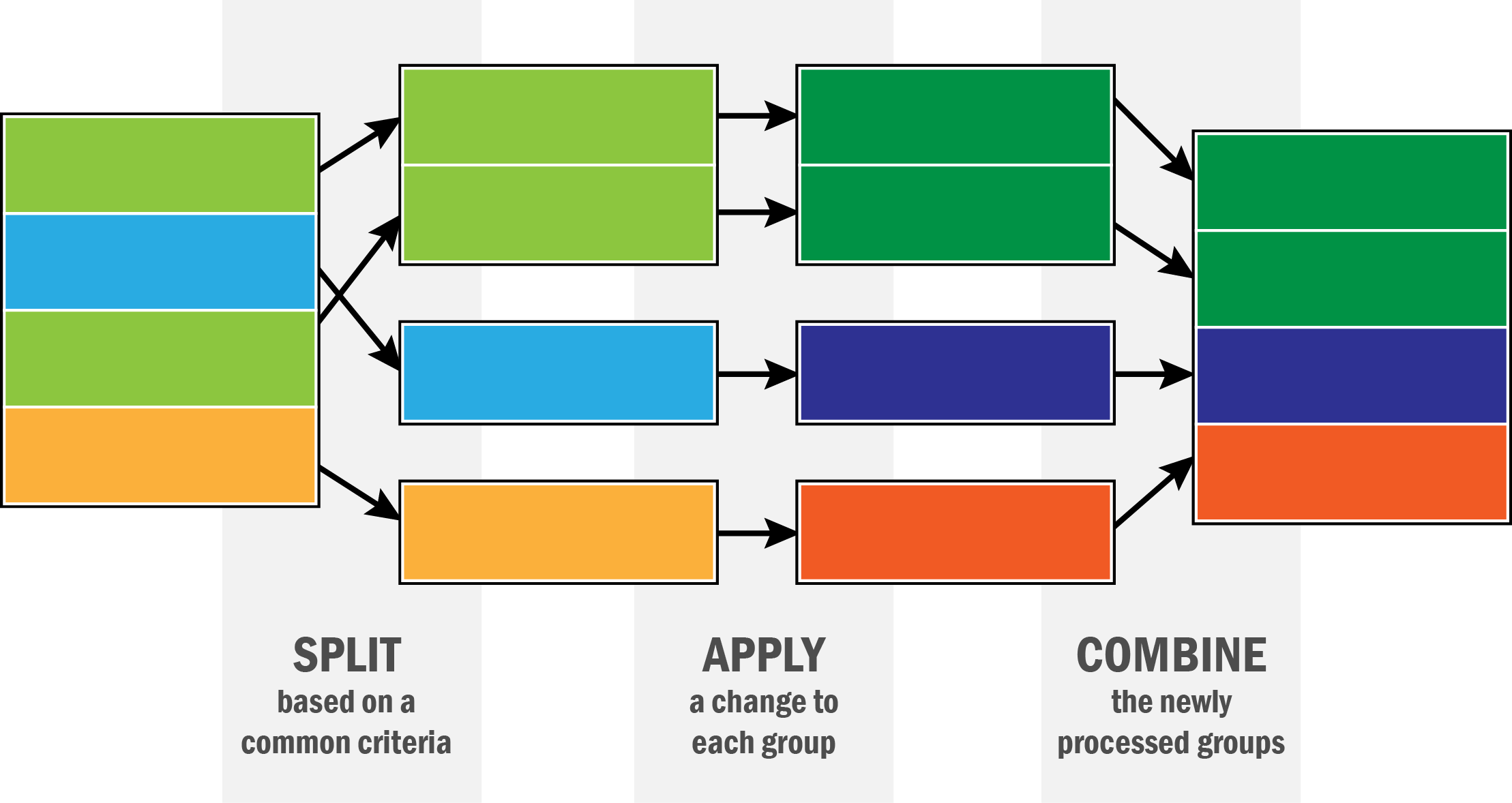

---

![](img/split-apply-combine.png)

---

# Grouped summaries

```r
mtcars1 %>% 
  group_by(cyl) %>% 
  summarize(mpg_mean = mean(mpg))
```

```
# A tibble: 3 x 2
  cyl   mpg_mean
  <fct>    <dbl>
1 4         26.7
2 6         19.7
3 8         15.1
```

---

# Grouped summaries

```r
mtcars1 %>% 
  group_by(cyl) %>% 
  summarize_if(is.numeric, mean)
```

```
# A tibble: 3 x 7
  cyl     mpg  disp    hp  drat    wt  qsec
  <fct> <dbl> <dbl> <dbl> <dbl> <dbl> <dbl>
1 4      26.7  105.  82.6  4.07  2.29  19.1
2 6      19.7  183. 122.   3.59  3.12  18.0
3 8      15.1  353. 209.   3.23  4.00  16.8
```

---

# Grouped summaries

```r
mtcars1 %>% 
  group_by(cyl) %>% 
  summarize_if(is.numeric, list('mean' = mean, 'median' = median))
```

```
# A tibble: 3 x 13
  cyl   mpg_mean disp_mean hp_mean drat_mean wt_mean qsec_mean mpg_median
  <fct>    <dbl>     <dbl>   <dbl>     <dbl>   <dbl>     <dbl>      <dbl>
1 4         26.7      105.    82.6      4.07    2.29      19.1       26  
2 6         19.7      183.   122.       3.59    3.12      18.0       19.7
3 8         15.1      353.   209.       3.23    4.00      16.8       15.2
# … with 5 more variables: disp_median <dbl>, hp_median <dbl>,
#   drat_median <dbl>, wt_median <dbl>, qsec_median <dbl>
```

---

# Foreign aid (DOS)

```r
dos %>% 
  group_by(Implementing_Organization) %>% 
  summarize(amt = sum(Award_Transaction_Value)) %>% 
  arrange(desc(amt))
```

```
# A tibble: 9,236 x 2
   Implementing_Organization                        amt
   <chr>                                          <dbl>
 1 United Nations High Commission           9548068186 
 2 ""                                       3374123507.
 3 Information Redacted                     3046872292.
 4 Un Relief & Works Agency                 2975220114 
 5 Intl Committee - The Red Cross           2796820000 
 6 S/S-Ex Miscellanous Vendor               2433986355.
 7 International Organization For Migration 1886668868.
 8 P A E                                     961874214.
 9 Pm Miscellaneous  Vendor                  925306561.
10 Un Childrens Fund                         775056737.
# … with 9,226 more rows
```

---
# Foreign aid (DOS)

```r
dos %>% 
  group_by(Implementing_Organization_Type) %>% 
  summarize(amt = sum(Award_Transaction_Value)) %>% 
  arrange(desc(amt))
```

```
# A tibble: 4 x 2
  Implementing_Organization_Type          amt
  <chr>                                 <dbl>
1 ""                             36464252937.
2 Other Public Sector             4522645303.
3 Government                       730826152.
4 Private Sector                   714436474.
```

---
# Foreign aid (DOS)

```r
dos %>% 
  group_by(Implementing_Organization, year = year(as_date(Award_Start_Date))) %>% 
  summarize(amt = sum(Award_Transaction_Value)) %>% 
  filter(Implementing_Organization != '', !is.na(year)) 
```

```
# A tibble: 3,907 x 3
# Groups:   Implementing_Organization [2,098]
   Implementing_Organization                                  year      amt
   <chr>                                                     <dbl>    <dbl>
 1 'Bsk-Asia' Llp                                             2015   1.53e5
 2 'Terratech' Ltd.                                           2015   2.59e5
 3 (Foreign Parent Is Institute For International Research …  2013   6.27e3
 4 (Foreign Parent Is Open Text Corporation, Waterloo, Cana…  2012   7.91e4
 5 3m Cogent, Inc.                                            2016   1.29e6
 6 5 GYRES INSTITUTE, THE                                     2016  -1.24e5
 7 A + P Consultants                                          2012   3.96e5
 8 A + P Consultants                                          2013   8.75e4
 9 A + P Consultants                                          2014   6.65e4
10 A Call To Serve Missouri                                   2013   6.70e5
# … with 3,897 more rows
```

Save this as `dos_by_year`.

---
# Foreign aid (DOS)

```r
dos_by_year %>% 
  group_by(year) %>% 
  summarize(amt = sum(amt))
```

```
# A tibble: 17 x 2
    year           amt
   <dbl>         <dbl>
 1  2002        24162 
 2  2003         4350 
 3  2004      -211515.
 4  2005     24294032.
 5  2006        65101.
 6  2007     30762236.
 7  2008     28449918.
 8  2009    142067481.
 9  2010     11081559.
10  2011   1482727259.
11  2012   7703229189.
12  2013  10598445712.
13  2014   9672512696.
14  2015   6228419232.
15  2016    915449161.
16  2017    860274841.
17  2018      2327908 
```